The Exponential Family and Generalized Linear Models

Linear regression and logistic regression are not two separate inventions; they are two turns of one crank. This post builds the exponential family and generalized linear models from first principles, shows why the sigmoid is inevitable, solves a brand-new problem (counting customers) almost for free, and derives softmax regression, all from a single recipe.

Where We Left Off

In the linear regression post, we learned to predict a continuous number: given the features of a house, how many dollars is it worth? We modeled the output as the linear prediction plus Gaussian noise, \(y \mid \vb{x} \sim \mathcal{N}\left(\mu, \sigma^2\right)\) with \(\mu = \boldsymbol{\uptheta}^{\intercal}\vb{x}\), and out fell least-squares regression.

In the classification post, we learned to predict a yes-or-no label: is this tumor malignant? We modeled the output as Bernoulli, \(y \mid \vb{x} \sim \operatorname{Bernoulli}\left(\phi\right)\) with \(\phi = g\left(\boldsymbol{\uptheta}^{\intercal}\vb{x}\right)\), where \(g\) was the sigmoid, and out fell logistic regression.

Those two posts left three loose ends dangling, and I promised we would come back for them:

1. Why the sigmoid? In logistic regression we reached for the function \(g\left(z\right) = 1 / \left(1 + e^{-z}\right)\) seemingly out of thin air. We wanted something that squashes any real number into \(\left[0, 1\right]\), and the sigmoid did the job, but why that function and not some other S-shaped curve?
2. Why the same update rule? Linear regression, the perceptron, and logistic regression all ended up trained by the identical rule \(\boldsymbol{\uptheta} \leftarrow \boldsymbol{\uptheta} + \alpha\left(y_i - h_{\boldsymbol{\uptheta}}\left(\vb{x}_i\right)\right)\vb{x}_i\). Three different stories, one update. That cannot be a coincidence.
3. What about other kinds of output? Suppose the thing we want to predict is neither a real number nor a binary label.

Let me make that third point concrete, because it is the itch this whole post scratches.

A coffee shop, and a data type we cannot handle yet

Imagine you run a small coffee shop. You already own two machine learning tools. Linear regression predicts your revenue next hour (a continuous number, say \(\$83.40\)). Logistic regression predicts whether a given first-time visitor will come back (a yes/no). Business is good.

Now your landlord asks a new question: how many customers will walk in next hour? The answer is a count: \(0, 1, 2, 3, \ldots\) It is a whole number, and it can never be negative.

Try your existing tools on it and both misbehave:

• Linear regression happily predicts \(-2.3\) customers, which is nonsense, and it assumes the noise is a symmetric Gaussian, whereas counts are lopsided (you can undershoot \(5\) by at most \(5\), but you can overshoot it without limit).
• Logistic regression is built for exactly two outcomes. It has no idea what to do with “\(7\)”.

So here is the uncomfortable question. Every time the type of thing we predict changes (real number, yes/no, count, category, waiting time), must we invent a brand-new algorithm from scratch: pick a distribution, write out its likelihood, take derivatives by hand, and derive a fresh update rule?

The answer, and the whole point of this post, is no. There is a single recipe. You pick the probability distribution that matches your data’s type, you turn a mechanical crank, and out comes a complete algorithm, hypothesis function and update rule included. Linear regression and logistic regression are just this recipe run with two different distributions. That recipe is the generalized linear model (GLM), and the language that makes it work is the exponential family of distributions.

By the end, the sigmoid will no longer look arbitrary (it will be forced on us the moment we say “Bernoulli”), the shared update rule will be explained (it is a theorem, not a coincidence), and the coffee-shop counting problem will be solved almost for free.

This post is largely based on the treatment in Ng & Ma (2023) and the accompanying lecture by Anand Avati in the Stanford CS229 series (Stanford Online, Anand Avati, 2019). The generalized linear model framework was developed in depth by McCullagh & Nelder (1989); for background on the exponential family, see Bishop (2006, Chapter 4) and Hastie et al. (2009).

Here is the journey ahead.

flowchart TB
    A["<b>1. A New Data Type</b><br/>Counts: how many<br/>customers next hour?"]
    B["<b>2. Two Clues</b><br/>What linear and logistic<br/>regression secretly share"]
    C["<b>3. The Exponential Family</b><br/>One form, many<br/>distributions"]
    D["<b>4. Two Gifts</b><br/>Convex loss,<br/>easy mean and variance"]
    E["<b>5. The GLM Recipe</b><br/>Three assumptions"]
    F["<b>6. Turning the Crank</b><br/>Recover OLS and<br/>logistic regression"]
    G["<b>7. Three Parameters</b><br/>Model, natural, mean"]
    H["<b>8. The Zoo of GLMs</b><br/>One update rule<br/>for all"]
    I["<b>9. Softmax Regression</b><br/>Many classes at once"]
    J["<b>10. Wrapping Up</b><br/>The full picture"]
    A --> B --> C --> D --> E --> F --> G --> H --> I --> J

    style A fill:#1e8449,color:#fff,stroke:#fff
    style H fill:#1f6f8b,color:#fff,stroke:#fff
    style J fill:#b9770e,color:#fff,stroke:#fff

We start by looking hard at the two tools we already trust, to find the pattern hiding inside them.

Two Clues Hiding in Plain Sight

Put linear regression and logistic regression side by side and stare at them.

Linear regression

\[ y \mid \vb{x}; \boldsymbol{\uptheta} \sim \mathcal{N}\left(\mu, \sigma^2\right) \]

\[ h_{\boldsymbol{\uptheta}}\left(\vb{x}\right) = \mu = \boldsymbol{\uptheta}^{\intercal}\vb{x} \]

Logistic regression

\[ y \mid \vb{x}; \boldsymbol{\uptheta} \sim \operatorname{Bernoulli}\left(\phi\right) \]

\[ h_{\boldsymbol{\uptheta}}\left(\vb{x}\right) = \phi = g\left(\boldsymbol{\uptheta}^{\intercal}\vb{x}\right) = \frac{1}{1 + e^{-\boldsymbol{\uptheta}^{\intercal} \vb{x}}} \]

Two clues jump out.

• Clue 1: each model picks a distribution for \(y \mid \vb{x}\) based on the type of \(y\). When \(y\) is a real number, we reached for the Gaussian. When \(y\) is binary, we reached for the Bernoulli. The choice was driven entirely by the kind of value \(y\) can take. It makes no sense to put a Bernoulli on a house price, or a Gaussian on a coin flip. The data type chose the distribution.
• Clue 2: both models push the same quantity \(\boldsymbol{\uptheta}^{\intercal}\vb{x}\) through some function to produce the mean of that distribution. In both cases the hypothesis \(h_{\boldsymbol{\uptheta}}\left(\vb{x}\right)\) is the mean of the distribution we chose (\(\mu\) for the Gaussian, \(\phi\) for the Bernoulli). The only difference is the function we apply to \(\boldsymbol{\uptheta}^{\intercal}\vb{x}\) on the way there: the identity function for linear regression, the sigmoid for logistic regression.

And recall the third clue from the last post, the one we could not explain: both are trained by the identical update rule

\[ \boldsymbol{\uptheta} \leftarrow \boldsymbol{\uptheta} + \alpha\left(y_i - h_{\boldsymbol{\uptheta}}\left(\vb{x}_i\right)\right)\vb{x}_i. \]

Three clues, all pointing at the same hidden structure. To see it, we need a language general enough to talk about “the Gaussian, the Bernoulli, and many friends” all at once, and in particular to talk about the mean of any of them in a uniform way. That language is the exponential family.

The Exponential Family: One Form for Many Distributions

Here is the definition. It looks cryptic at first; we will add color to every piece immediately after.

We say a class of distributions belongs to the exponential family if its probability density (for a continuous \(y\)) or probability mass function (for a discrete \(y\)) can be written in the form

\[ p\left(y; \eta\right) = b\left(y\right)\exp\left(\eta \, T\left(y\right) - a\left(\eta\right)\right). \tag{1}\]

Every symbol has a name and a job:

• \(\eta\) is the natural parameter (also called the canonical parameter). It is the single knob that indexes the distributions in the family: as you dial \(\eta\), you sweep through the members.
• \(T\left(y\right)\) is the sufficient statistic. For every distribution we will meet in this post, it is simply \(T\left(y\right) = y\), so you can mentally read it as “\(y\)” and lose nothing.
• \(b\left(y\right)\) is the base measure. It depends on \(y\) alone, with no \(\eta\) in it.
• \(a\left(\eta\right)\) is the log partition function. It depends on \(\eta\) alone, with no \(y\) in it.

The one piece worth dwelling on is \(a\left(\eta\right)\). Its job is bookkeeping: it is exactly what makes the whole expression a valid probability distribution, one that sums or integrates to \(1\) over all \(y\). To see why, notice that if we drop the \(-a\left(\eta\right)\) term, the leftover \(b\left(y\right)\exp\left(\eta \, T\left(y\right)\right)\) is some non-negative function of \(y\), but there is no reason for it to sum to \(1\). So we divide by whatever it sums to. That normalizing total is \(e^{a\left(\eta\right)}\), and dividing by it is the same as subtracting \(a\left(\eta\right)\) inside the exponent. In symbols,

\[ e^{a\left(\eta\right)} = \sum_{y} b\left(y\right)\exp\left(\eta \, T\left(y\right)\right) \quad \text{(or } \int \text{ for continuous } y\text{)}, \]

so \(a\left(\eta\right)\) is the logarithm of the normalizing total, which is exactly why it is called the log partition function. (“Partition function” is borrowed from statistical physics, where normalizing constants go by that name.)

NoteOptional sidebar: where the names come from (exponential tilting)

Here is a nice way to see the family being built, which explains all the terminology at once. Start with any non-negative function \(b\left(y\right)\) (the “base measure”, before any parameter is involved). Now introduce a parameter \(\eta\) and multiply pointwise by \(e^{\eta \, y}\), then renormalize:

\[ p\left(y; \eta\right) = \frac{b\left(y\right)e^{\eta y}}{\displaystyle\int b\left(y\right)e^{\eta y}\,\dd{y}}. \]

This operation, nudging a base distribution by an exponential factor, is called exponential tilting. The denominator is just the number that makes it integrate to \(1\); taking its logarithm gives \(a\left(\eta\right)\). Every member of the exponential family is a tilted version of its base measure. (This sidebar is pure motivation; nothing later depends on it, so skip it freely.)

That is the abstract form. The claim, and the reason the family matters, is that a great many everyday distributions can be massaged into Equation 1. Let us do it for the two we already care about. The technique both times is the same: take the familiar formula, rewrite it as \(\exp\left(\log\left(\cdots\right)\right)\), and pattern-match against Equation 1 to read off \(\eta\), \(T\), \(a\), and \(b\). Nothing more than algebra is involved.

The Bernoulli is in the family (and the sigmoid appears)

The Bernoulli distribution with mean \(\phi\) puts probability \(\phi\) on \(y = 1\) and \(1 - \phi\) on \(y = 0\). We can write both cases in one line as \(p\left(y; \phi\right) = \phi^{y}\left(1 - \phi\right)^{1 - y}\). Now the massaging:

\[ \begin{align*} p\left(y; \phi\right) &= \phi^{y}\left(1 - \phi\right)^{1 - y}\\ &= \exp\left(y \log \phi + \left(1 - y\right)\log\left(1 - \phi\right)\right)\\ &= \exp\left(\log\left(\frac{\phi}{1 - \phi}\right)\, y + \log\left(1 - \phi\right)\right)\\ &= \exp\bigg(\underbrace{\log\left(\frac{\phi}{1 - \phi}\right)}_{\eta}\, y + \underbrace{\log\left(1 - \phi\right)}_{-a\left(\eta\right)}\bigg). \end{align*} \]

Pattern-matching against Equation 1, we read off the four pieces:

\[ \eta = \log\left(\frac{\phi}{1 - \phi}\right), \qquad T\left(y\right) = y, \qquad a\left(\eta\right) = -\log\left(1 - \phi\right), \qquad b\left(y\right) = 1. \]

Now look at that first equation, the one defining the natural parameter \(\eta\) in terms of the mean \(\phi\). What if we invert it, solving for \(\phi\) in terms of \(\eta\)? Starting from \(\eta = \log\left(\phi / \left(1 - \phi\right)\right)\), exponentiate and rearrange:

\[ e^{\eta} = \frac{\phi}{1 - \phi} \implies \phi = \frac{1}{1 + e^{-\eta}}. \]

That is the sigmoid. It was not chosen; it fell out of the algebra the instant we asked “how does the Bernoulli’s mean relate to its natural parameter?” This is the first promised loose end, tied off: once you decide to model \(y\) as Bernoulli, the sigmoid is not a design choice you make, it is a consequence you discover. (We will make this precise in Section 6, where it becomes the hypothesis of logistic regression.)

For completeness, we can also rewrite \(a\left(\eta\right)\) purely in terms of \(\eta\). Manipulating the first equation we got after pattern matching gives us

\[ 1 - \phi = \frac{1}{\left(1 + e^{\eta}\right)}. \]

Substituting this in the third equation obtained after pattern matching, we get

\[ a\left(\eta\right) = -\log\left(1 - \phi\right) = -\log\left(\frac{1}{\left(1 + e^{\eta}\right)}\right) = \log\left(1 + e^{\eta}\right). \]

The Gaussian is in the family too

Recall that when we derived linear regression, the variance \(\sigma^2\) dropped out of the final answer for \(\boldsymbol{\uptheta}\): it did not affect our choice of hypothesis at all. So we are free to fix it at any convenient value, and \(\sigma^2 = 1\) makes the algebra cleanest. With that, the Gaussian density is

\[ p\left(y; \mu\right) = \frac{1}{\sqrt{2\pi}}\exp\left(-\frac{1}{2}\left(y - \mu\right)^2\right). \]

Expand the square and split off the part that depends only on \(y\):

\[ \begin{align*} p\left(y; \mu\right) &= \frac{1}{\sqrt{2\pi}}\exp\left(-\frac{1}{2}\left(y - \mu\right)^2\right)\\ &= \frac{1}{\sqrt{2\pi}}\exp\left(-\frac{1}{2}y^2\right)\,\exp\left(\mu y - \frac{1}{2}\mu^2\right)\\ &= \underbrace{\frac{1}{\sqrt{2\pi}}\exp\left(-\frac{1}{2}y^2\right)}_{b\left(y\right)}\,\exp\bigg(\underbrace{\mu}_{\eta}\, y - \underbrace{\frac{1}{2}\mu^2}_{a\left(\eta\right)}\bigg). \end{align*} \]

Pattern-matching once more against Equation 1:

\[ \eta = \mu, \qquad T\left(y\right) = y, \qquad a\left(\eta\right) = \frac{\mu^2}{2} = \frac{\eta^2}{2}, \qquad b\left(y\right) = \frac{1}{\sqrt{2\pi}}\exp\left(-\frac{y^2}{2}\right). \]

Here the relationship between the natural parameter and the mean is as simple as it gets: \(\eta = \mu\). The mean is the natural parameter. Hold on to that; it is what will make linear regression fall out in Section 6.

These two are not special. The Poisson (for counts, which is exactly our coffee-shop problem), the exponential and gamma (for waiting times), the beta and Dirichlet (for probabilities), the categorical (for one-of-\(k\) labels), and many more are all members. Each is just a different choice of \(T\), \(a\), and \(b\). In the next section we cash in that generality.

Two Gifts the Family Gives Us

Before building the recipe, it is worth pausing to appreciate why the exponential family is the right abstraction. Writing a distribution in the form of Equation 1 buys us two properties that hold for every member at once. We will state and interpret them, and then derive both. Remarkably, both fall out of a single humble fact: that a probability distribution must sum (or integrate) to \(1\).

Gift 1: the log-likelihood is concave in \(\eta\)

Equivalently, the negative log-likelihood, which is the loss we minimize, is convex. This is the property that makes learning well-behaved: a convex loss has no bad local minima to get stuck in, so gradient descent (and Newton’s method, from the last post) marches to the single global optimum. When we later set \(\eta = \boldsymbol{\uptheta}^{\intercal}\vb{x}\), the loss stays convex as a function of \(\boldsymbol{\uptheta}\), because plugging a linear function of \(\boldsymbol{\uptheta}\) into a convex function keeps it convex. This is the deep reason the logistic regression log-likelihood was concave, a fact we used but did not justify last time. And as we are about to see, it is not even a separate miracle: it follows in one line from Gift 2.

Gift 2: the mean and variance are just derivatives of \(a\left(\eta\right)\)

Specifically,

\[ \mathbb{E}\left[y; \eta\right] = \dv{a}{\eta}, \qquad \operatorname{Var}\left[y; \eta\right] = \dv[2]{a}{\eta}. \]

Normally, computing a mean means grinding through an integral \(\int y \, p\left(y\right)\dd{y}\), and a variance is worse. For the exponential family, you just differentiate the log partition function. This is not only convenient; it is the bridge we need, because the whole GLM idea rests on predicting the mean, and this tells us the mean is \(a'\left(\eta\right)\).

It is worth checking these on the cases we just derived, both to build trust and because we will reuse the results.

Bernoulli: \(a\left(\eta\right) = \log\left(1 + e^{\eta}\right)\)

\[ a'\left(\eta\right) = \frac{e^{\eta}}{1 + e^{\eta}} = \frac{1}{1 + e^{-\eta}} = \phi. \]

The derivative of \(a\) is exactly the mean \(\phi\), and it is exactly the sigmoid again.

Gaussian: \(a\left(\eta\right) = \dfrac{\eta^2}{2}\)

\[ a'\left(\eta\right) = \eta = \mu. \]

The derivative of \(a\) is exactly the mean \(\mu\).

Both check out: differentiating \(a\left(\eta\right)\) hands back the mean, with no integral in sight. Keep Section 4 in mind; Gift 2 is about to do all the heavy lifting.

Where the two gifts come from

Neither gift is magic. Both flow from the one fact every distribution must obey: it sums (or integrates) to \(1\). Foreshadowing the destination, we will differentiate that normalization statement once to get the mean, differentiate again to get the variance, and then read off the concavity for free. Here is the whole thing.

The normalization condition for Equation 1 says that, for every value of \(\eta\),

\[ \int b\left(y\right)\exp\left(\eta \, T\left(y\right) - a\left(\eta\right)\right)\dd{y} = 1 \tag{2}\]

(with a sum in place of the integral when \(y\) is discrete). The trick is that this holds identically in \(\eta\), so we may differentiate both sides with respect to \(\eta\) and the right-hand side stays \(0\). Differentiating the integrand brings down a factor \(\left(T\left(y\right) - a'\left(\eta\right)\right)\), and the bracketed quantity that multiplies it is just \(p\left(y; \eta\right)\) again:

\[ \int \underbrace{b\left(y\right)\exp\left(\eta \, T\left(y\right) - a\left(\eta\right)\right)}_{p\left(y; \eta\right)}\left(T\left(y\right) - a'\left(\eta\right)\right)\dd{y} = 0. \]

Split the integral into two, and use \(\int p\left(y; \eta\right)\dd{y} = 1\) on the second piece:

\[ \int p\left(y; \eta\right)T\left(y\right)\dd{y} - a'\left(\eta\right) = 0 \implies \mathbb{E}\left[T\left(y\right); \eta\right] = a'\left(\eta\right). \]

That is the mean half of Gift 2. Now differentiate that last integral identity with respect to \(\eta\) one more time. Differentiating the \(p\left(y; \eta\right)\) factor again produces another \(\left(T\left(y\right) - a'\left(\eta\right)\right)\), while differentiating the explicit \(\left(T\left(y\right) - a'\left(\eta\right)\right)\) gives \(-a''\left(\eta\right)\):

\[ \int p\left(y; \eta\right)\left[\left(T\left(y\right) - a'\left(\eta\right)\right)^2 - a''\left(\eta\right)\right]\dd{y} = 0. \]

The first term is the average squared deviation of \(T\left(y\right)\) from its mean \(a'\left(\eta\right)\), which is exactly the variance; the second term is a constant that pulls out of the integral. Rearranging,

\[ \operatorname{Var}\left[T\left(y\right); \eta\right] = a''\left(\eta\right), \]

the variance half of Gift 2.

Gift 1 now comes for free. The log-likelihood of one example is \(\log p\left(y; \eta\right) = \log b\left(y\right) + \eta \, T\left(y\right) - a\left(\eta\right)\). The first term has no \(\eta\) and the second is linear in \(\eta\), so both vanish under a second derivative, leaving

\[ \dv[2]{\eta}\log p\left(y; \eta\right) = -a''\left(\eta\right) = -\operatorname{Var}\left[T\left(y\right); \eta\right] \leq 0, \]

because a variance can never be negative. A function whose second derivative is never positive is concave, so the log-likelihood is concave in \(\eta\), and its negative (the loss) is convex. That is Gift 1, and notice it was not a separate fact at all: it is Gift 2 plus the observation that variances are non-negative.

Let us take stock before assembling the recipe.

flowchart TB
    A["<b>1. A New Data Type</b>"]
    B["<b>2. Two Clues</b>"]
    C["<b>3. The Exponential Family</b>"]
    D["<b>4. Two Gifts</b><br/>Convex loss,<br/>easy mean and variance"]
    E["<b>5. The GLM Recipe</b>"]
    F["<b>6. Turning the Crank</b>"]
    G["<b>7. Three Parameters</b>"]
    H["<b>8. The Zoo of GLMs</b>"]
    I["<b>9. Softmax Regression</b>"]
    J["<b>10. Wrapping Up</b>"]
    A --> B --> C --> D --> E --> F --> G --> H --> I --> J

    style D fill:#c0392b,color:#fff,stroke:#fff

We now have a common language (the exponential family) and a way to get any member’s mean cheaply (Gift 2). Time to connect this machinery to the inputs \(\vb{x}\).

The GLM Recipe: Three Assumptions

So far the exponential family has been a statement about a lone variable \(y\) and its parameter \(\eta\); there has been no \(\vb{x}\) anywhere. But supervised learning is about a mapping from inputs \(\vb{x}\) to outputs \(y\). A generalized linear model bridges the two with exactly three assumptions. Think of them as the three steps of the recipe.

1. Choose the distribution. Assume \(y \mid \vb{x}; \boldsymbol{\uptheta} \sim \text{ExponentialFamily}\left(\eta\right)\). That is, given the input, the output follows some exponential-family distribution with natural parameter \(\eta\). Which member you pick is dictated by the data type of \(y\) (this is Clue 1 from earlier, now promoted to step one of the recipe).
2. Predict the mean. Our hypothesis should output the expected value of \(y\) given \(\vb{x}\): \[ h_{\boldsymbol{\uptheta}}\left(\vb{x}\right) = \mathbb{E}\left[y \mid \vb{x}; \boldsymbol{\uptheta}\right]. \] This is a reasonable thing to want: if you know \(y\)’s distribution and must commit to a single prediction, its mean is a natural choice. (This is Clue 2.)
3. Tie the natural parameter to the input, linearly. Assume \[ \eta = \boldsymbol{\uptheta}^{\intercal}\vb{x} \] (and if \(\eta\) is vector-valued, then \(\eta_i = \boldsymbol{\uptheta}_i^{\intercal}\vb{x}\), one linear predictor per component).

The third assumption is less a law of nature than a design choice, and it is where the word “linear” in “generalized linear model” comes from. We decide to make the natural parameter a linear function of the features. Nothing stops you from making it something fancier, say \(\eta = \left(\text{a neural network}\right)\left(\vb{x}\right)\); you would then have a perfectly good model, just no longer a linear one. (File that thought away: it is a first glimpse of where neural networks come from.)

These three steps describe a data-generating process, a story for how each \(\left(\vb{x}_i, y_i\right)\) pair came to be. Figure 1 draws that story as a pipeline.

Figure 1: The GLM as a data-generating pipeline. The global model parameters \(\boldsymbol{\theta}\) (trained once, shared across all examples) dot with an input \(\mathbf{x}_i\) to produce that example’s natural parameter \(\eta_i\). Choosing the distribution fixes \(\left(T, a, b\right)\) and hence the canonical response function \(g\), which maps \(\eta_i\) to the mean parameter; that mean is our prediction \(h_{\boldsymbol{\theta}}\left(\mathbf{x}_i\right)\). Finally \(y_i\) is a sample from the resulting distribution.

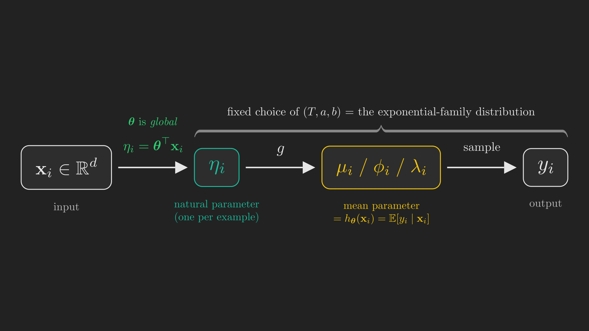
Two things in Figure 1 are worth stating out loud, because they are easy to conflate:

• The model parameters \(\boldsymbol{\uptheta}\) are global: there is one \(\boldsymbol{\uptheta}\) for the entire model, and training adjusts it.
• The natural parameter \(\eta_i = \boldsymbol{\uptheta}^{\intercal}\vb{x}_i\) is per-example: every input produces its own \(\eta_i\), and hence its own distribution to sample \(y_i\) from.

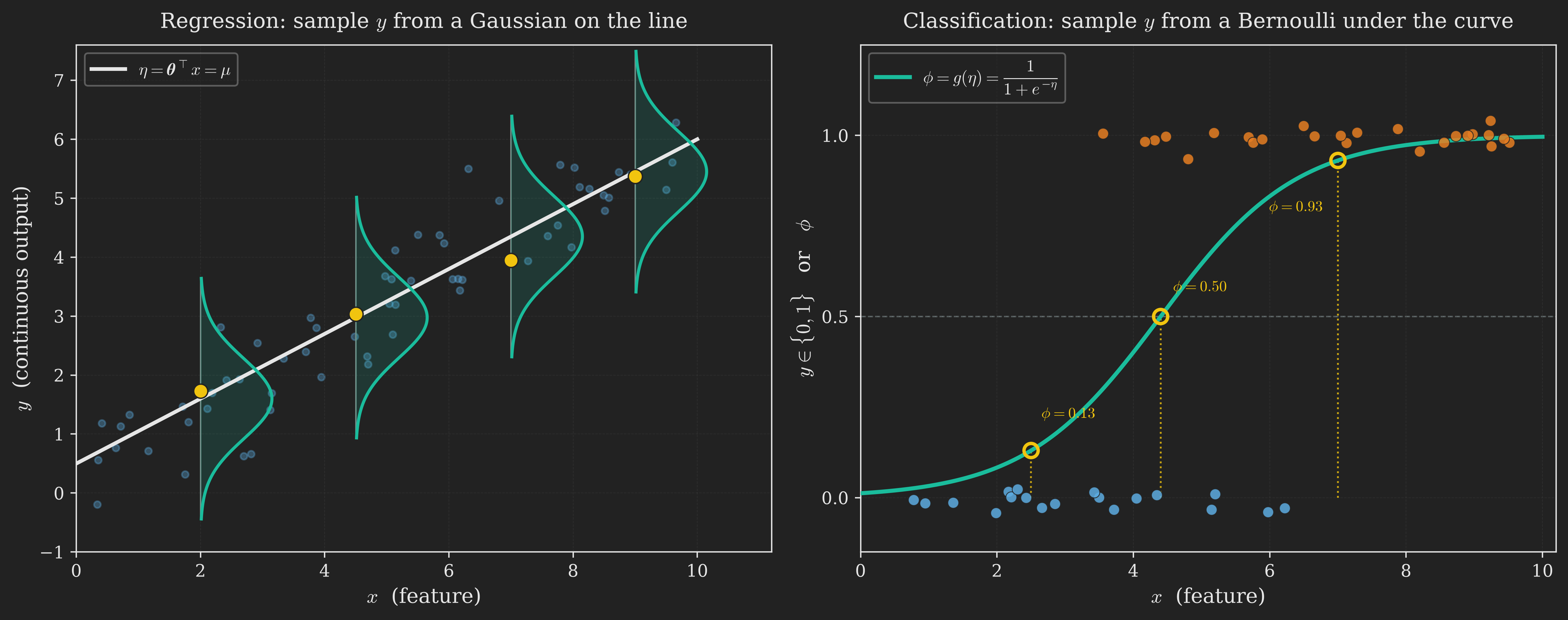
To make this pipeline less abstract, Figure 2 shows the data-generating story for the two distributions we already know. Read each panel left to right along the input axis: at every \(x\), the model builds a little distribution (a Gaussian or a Bernoulli), and the observed \(y\) is a sample from it. Regression and classification are the same idea with a different distribution stood up at each point.

Figure 2: The GLM as a data-generating story, for the two cases we already know. Left (regression, Gaussian): at each input \(x\), the line \(\eta = \boldsymbol{\theta}^\top x = \mu\) sets the center of a Gaussian (the sideways bells), and the observed output (yellow) is a sample from it. Right (classification, Bernoulli): at each input \(x\), the sigmoid sets the success probability \(\phi = g\left(\eta\right)\), and the observed label (a \(0\) or a \(1\)) is a sample from a \(\operatorname{Bernoulli}\left(\phi\right)\); larger \(x\) makes a \(1\) more likely.

With the recipe in hand, let us turn the crank on our two familiar distributions and watch the algorithms we already know pop out.

Turning the Crank: Recovering What We Know

Ordinary least squares, from the Gaussian

Choose the Gaussian in step 1 (appropriate when \(y\) is a continuous real number). Then the hypothesis is forced by the three assumptions, one equality at a time:

\[ \begin{align*} h_{\boldsymbol{\uptheta}}\left(\vb{x}\right) &= \mathbb{E}\left[y \mid \vb{x}; \boldsymbol{\uptheta}\right] && \text{(step 2: predict the mean)}\\ &= \mu && \text{(the mean of a Gaussian is } \mu\text{)}\\ &= \eta && \text{(for the Gaussian, } \eta = \mu\text{)}\\ &= \boldsymbol{\uptheta}^{\intercal}\vb{x}. && \text{(step 3: } \eta = \boldsymbol{\uptheta}^{\intercal}\vb{x}\text{)} \end{align*} \]

We recover \(h_{\boldsymbol{\uptheta}}\left(\vb{x}\right) = \boldsymbol{\uptheta}^{\intercal}\vb{x}\), the linear regression hypothesis, with no further invention.

Logistic regression, from the Bernoulli

Choose the Bernoulli in step 1 (appropriate when \(y\) is binary). Recall from our derivation above that the Bernoulli’s mean and natural parameter are linked by \(\phi = 1 / \left(1 + e^{-\eta}\right)\), and that the mean of a \(\operatorname{Bernoulli}\left(\phi\right)\) is \(\phi\) itself. Then:

\[ \begin{align*} h_{\boldsymbol{\uptheta}}\left(\vb{x}\right) &= \mathbb{E}\left[y \mid \vb{x}; \boldsymbol{\uptheta}\right] && \text{(step 2: predict the mean)}\\ &= \phi && \text{(the mean of a Bernoulli is } \phi\text{)}\\ &= \frac{1}{1 + e^{-\eta}} && \text{(for the Bernoulli, } \phi = 1 / \left(1 + e^{-\eta}\right)\text{)}\\ &= \frac{1}{1 + e^{-\boldsymbol{\uptheta}^{\intercal}\vb{x}}}. && \text{(step 3: } \eta = \boldsymbol{\uptheta}^{\intercal}\vb{x}\text{)} \end{align*} \]

There it is, in full: \(h_{\boldsymbol{\uptheta}}\left(\vb{x}\right) = 1 / \left(1 + e^{-\boldsymbol{\uptheta}^{\intercal}\vb{x}}\right)\), the logistic regression hypothesis. The sigmoid is not something we picked because it looked S-shaped; it is what the recipe hands you the moment you say “model \(y\) as Bernoulli.” The first loose end from the introduction is now fully tied off.

Naming the function in the middle

In both derivations, the crucial step was the function connecting the natural parameter \(\eta\) to the mean. That function deserves a name. The function \(g\) that maps the natural parameter to the distribution’s mean,

\[ g\left(\eta\right) = \mathbb{E}\left[T\left(y\right); \eta\right], \]

is called the canonical response function (recall that \(y\) is often called the response variable, hence the name). Its inverse, \(g^{-1}\), which maps the mean back to the natural parameter, is the canonical link function. From Section 4 we even know a formula for \(g\): it is \(g\left(\eta\right) = a'\left(\eta\right)\), the derivative of the log partition function.

So the canonical response function of the Gaussian is the identity, \(g\left(\eta\right) = \eta\), and the canonical response function of the Bernoulli is the sigmoid, \(g\left(\eta\right) = 1 / \left(1 + e^{-\eta}\right)\). Same \(g\) that appears as the arrow in the middle of Figure 1.

Three Parameters, One Picture

By now several Greek letters are flying around: \(\boldsymbol{\uptheta}\), \(\eta\), \(\mu\), \(\phi\), and soon \(\lambda\). It is easy to lose track of who is who. The cure is to notice that they come in exactly three kinds, and that Figure 1 already shows how they relate. Let us name the three kinds explicitly.

• The model parameters \(\boldsymbol{\uptheta} \in \mathbb{R}^{d}\). These are what training learns and what we store. They are global (one set for the whole model), and they are the parameters gradient descent adjusts at every step. When training ends, \(\boldsymbol{\uptheta}\) is the model.
• The natural parameter \(\eta_i = \boldsymbol{\uptheta}^{\intercal}\vb{x}_i\). This is ephemeral: one value per example, computed on the fly, never stored. It is the bridge from the model parameters to the specific distribution for example \(i\).
• The mean parameter, whose name depends on the distribution: \(\mu\) for the Gaussian, \(\phi\) for the Bernoulli, \(\lambda\) for the Poisson, and so on. This is the prediction itself, \(h_{\boldsymbol{\uptheta}}\left(\vb{x}_i\right) = \mathbb{E}\left[y_i \mid \vb{x}_i\right]\).

The two arrows between them are the two relationships you must keep straight:

\[ \underbrace{\boldsymbol{\uptheta}}_{\text{model}} \;\xrightarrow{\;\;\boldsymbol{\uptheta}^{\intercal}\vb{x}\;\;}\; \underbrace{\eta}_{\text{natural}} \;\xrightarrow{\;\;g\;\;}\; \underbrace{\mu \,/\, \phi \,/\, \lambda}_{\text{mean (the prediction)}}. \]

The first arrow is the linear step (assumption 3). The second arrow is the canonical response function \(g\) (which the choice of distribution fixes). Training moves \(\boldsymbol{\uptheta}\); prediction runs an input rightward through both arrows. If you ever feel lost among the symbols in what follows, come back to this line.

Let us recap our position on the map before collecting the payoff.

flowchart TB
    A["<b>1. A New Data Type</b>"]
    B["<b>2. Two Clues</b>"]
    C["<b>3. The Exponential Family</b>"]
    D["<b>4. Two Gifts</b>"]
    E["<b>5. The GLM Recipe</b>"]
    F["<b>6. Turning the Crank</b>"]
    G["<b>7. Three Parameters</b><br/>Model, natural, mean"]
    H["<b>8. The Zoo of GLMs</b>"]
    I["<b>9. Softmax Regression</b>"]
    J["<b>10. Wrapping Up</b>"]
    A --> B --> C --> D --> E --> F --> G --> H --> I --> J

    style G fill:#c0392b,color:#fff,stroke:#fff

We have recovered two old algorithms from one recipe. Now for the reason the recipe is worth having: it handles data types we have never seen, and it explains the mysterious shared update rule.

The Zoo of GLMs, and One Update Rule to Rule Them All

Here is the payoff. To build a model for a new problem, you do not start from scratch. You follow the recipe:

1. Look at the data type of \(y\) and pick an exponential-family distribution whose support matches it.
2. Express that distribution in exponential-family form to read off its canonical response function \(g\) (equivalently, differentiate its log partition function, \(g = a'\)).
3. Write the hypothesis \(h_{\boldsymbol{\uptheta}}\left(\vb{x}\right) = g\left(\boldsymbol{\uptheta}^{\intercal}\vb{x}\right)\), and train.

Different data types slot into different distributions, and each gives a named algorithm. Table 1 is the zoo.

Table 1: The GLM zoo. The data type of the output picks the distribution, and the recipe turns that distribution into an algorithm.

Data type of \(y\)	A coffee-shop example	Distribution	Resulting GLM
Real, \(\left(-\infty, \infty\right)\)	tomorrow’s revenue	Gaussian	linear regression
Binary, \(\left\{0, 1\right\}\)	will this visitor return?	Bernoulli	logistic regression
Count, \(\left\{0, 1, 2, \ldots\right\}\)	customers next hour	Poisson	Poisson regression
Category, \(\left\{1, \ldots, k\right\}\)	drink ordered: coffee / tea / juice	Categorical	softmax regression
Positive real (a duration)	time until a customer churns	Exponential, Gamma	survival analysis

TipA tiny warning about a name collision

The exponential distribution (a single member, good for waiting times) is easy to confuse with the exponential family (the whole club of distributions in Equation 1). The exponential distribution is one member of the exponential family. Different things, unfortunately similar names.

Cashing the coffee-shop check: Poisson regression

Remember the customers-per-hour problem that we could not touch at the start? Its data type is count, so the zoo sends us to the Poisson. Let us run the recipe and watch the problem dissolve. The Poisson probability mass function is

\[ p\left(y; \lambda\right) = \frac{\lambda^{y}e^{-\lambda}}{y!}, \]

for \(y \in \left\{0, 1, 2, \ldots\right\}\). Massage it into exponential-family form (Equation 1) the same way as before:

\[ \begin{align*} p\left(y; \lambda\right) &= \frac{\lambda^{y}e^{-\lambda}}{y!}\\ &= \frac{1}{y!}\exp\left(\log \lambda\, y - \lambda\right)\\ &= \underbrace{\frac{1}{y!}}_{b\left(y\right)}\exp\big(\underbrace{\log \lambda}_{\eta}\, y - \underbrace{\lambda}_{a\left(\eta\right)}\big). \end{align*} \]

So the natural parameter is \(\eta = \log \lambda\), which inverts to \(\lambda = e^{\eta}\). The canonical response function is therefore \(g\left(\eta\right) = e^{\eta}\) (and you can double-check via Gift 2: with \(a\left(\eta\right) = \lambda = e^{\eta}\), indeed \(a'\left(\eta\right) = e^{\eta} = \lambda\), the mean of a Poisson). The hypothesis writes itself:

\[ h_{\boldsymbol{\uptheta}}\left(\vb{x}\right) = \mathbb{E}\left[y \mid \vb{x}; \boldsymbol{\uptheta}\right] = \lambda = e^{\eta} = e^{\boldsymbol{\uptheta}^{\intercal}\vb{x}}. \]

That is Poisson regression, and notice it is exactly what we needed: \(e^{\boldsymbol{\uptheta}^{\intercal}\vb{x}}\) is always positive, so the model can never predict a negative customer count. We did not derive a new algorithm by hand; we picked “Poisson” and turned the crank. The coffee-shop problem is solved.

Why the update rule was always the same

Now the second loose end. Across linear regression, the perceptron, and logistic regression, training always reduced to

\[ \boldsymbol{\uptheta} \leftarrow \boldsymbol{\uptheta} + \alpha\left(y_i - h_{\boldsymbol{\uptheta}}\left(\vb{x}_i\right)\right)\vb{x}_i. \tag{3}\]

This is not a coincidence; it is a theorem about GLMs. For any GLM built with the canonical response function, maximizing the log-likelihood by gradient ascent gives exactly Equation 3. Only \(h_{\boldsymbol{\uptheta}}\) changes from model to model (identity, sigmoid, exponential, …); the shape of the update is fixed.

NoteOptional: the one-line reason the update rule is universal

Consider a single example with \(T\left(y\right) = y\) and \(\eta = \boldsymbol{\uptheta}^{\intercal}\vb{x}\). Its log-likelihood is \(\log p\left(y; \eta\right) = \log b\left(y\right) + \eta y - a\left(\eta\right)\). Differentiate with respect to \(\boldsymbol{\uptheta}\), using \(\pdv{\eta}{\boldsymbol{\uptheta}} = \vb{x}\) and, crucially, Gift 2 (\(a'\left(\eta\right)\) is the mean, which is \(h_{\boldsymbol{\uptheta}}\left(\vb{x}\right)\)):

\[ \pdv{\boldsymbol{\uptheta}}\log p\left(y; \eta\right) = \left(y - a'\left(\eta\right)\right)\vb{x} = \left(y - h_{\boldsymbol{\uptheta}}\left(\vb{x}\right)\right)\vb{x}. \]

Summing over the training set and taking a gradient-ascent step gives Equation 3. The magic ingredient is Gift 2: because the mean is \(a'\left(\eta\right)\), the derivative collapses into “target minus prediction, times input” every single time.

And prediction is uniform too: for a new input \(\vb{x}^{\star}\), the prediction is always \(\hat{y} = h_{\boldsymbol{\uptheta}}\left(\vb{x}^{\star}\right) = g\left(\boldsymbol{\uptheta}^{\intercal}\vb{x}^{\star}\right)\), whatever the distribution.

Let us mark the map once more, then tackle the one entry in the zoo that needs real new machinery: the categorical case.

flowchart TB
    A["<b>1. A New Data Type</b>"]
    B["<b>2. Two Clues</b>"]
    C["<b>3. The Exponential Family</b>"]
    D["<b>4. Two Gifts</b>"]
    E["<b>5. The GLM Recipe</b>"]
    F["<b>6. Turning the Crank</b>"]
    G["<b>7. Three Parameters</b>"]
    H["<b>8. The Zoo of GLMs</b><br/>One update rule for all"]
    I["<b>9. Softmax Regression</b>"]
    J["<b>10. Wrapping Up</b>"]
    A --> B --> C --> D --> E --> F --> G --> H --> I --> J

    style H fill:#c0392b,color:#fff,stroke:#fff

Softmax Regression: A GLM for Many Classes

Every GLM so far has produced a single number as its mean. But the categorical case is different: when \(y \in \left\{1, 2, \ldots, k\right\}\) (say, classifying an email as spam, personal, or work-related, or a coffee order as coffee, tea, or juice), the “mean” we need is a whole probability vector \(\left(\phi_1, \ldots, \phi_k\right)\), one probability per class, subject to \(\sum_{c=1}^{k}\phi_c = 1\). This is the one entry in the zoo that needs genuinely new gears, so let us build them, starting from geometry.

The geometric idea: one direction per class

Back in logistic regression, a single parameter vector \(\boldsymbol{\uptheta}\) carved the input space into two half-spaces: points with \(\boldsymbol{\uptheta}^{\intercal}\vb{x} > 0\) were one class, points with \(\boldsymbol{\uptheta}^{\intercal}\vb{x} < 0\) the other. For \(k\) classes, the natural generalization is to give each class its own parameter vector \(\boldsymbol{\uptheta}_c\), and to classify an input by whichever vector it aligns with best. Figure 3 shows the picture.

Figure 3: The geometry of multi-class classification. Each class \(c\) gets its own parameter vector \(\boldsymbol{\theta}_c\), drawn pointing toward that class’s cluster of examples. To classify an input \(\mathbf{x}\), we compute the score \(\boldsymbol{\theta}_c^{\intercal}\mathbf{x}\) for every class (a large score means \(\mathbf{x}\) aligns with, points in nearly the same direction as, that class’s vector) and predict the class with the largest score.

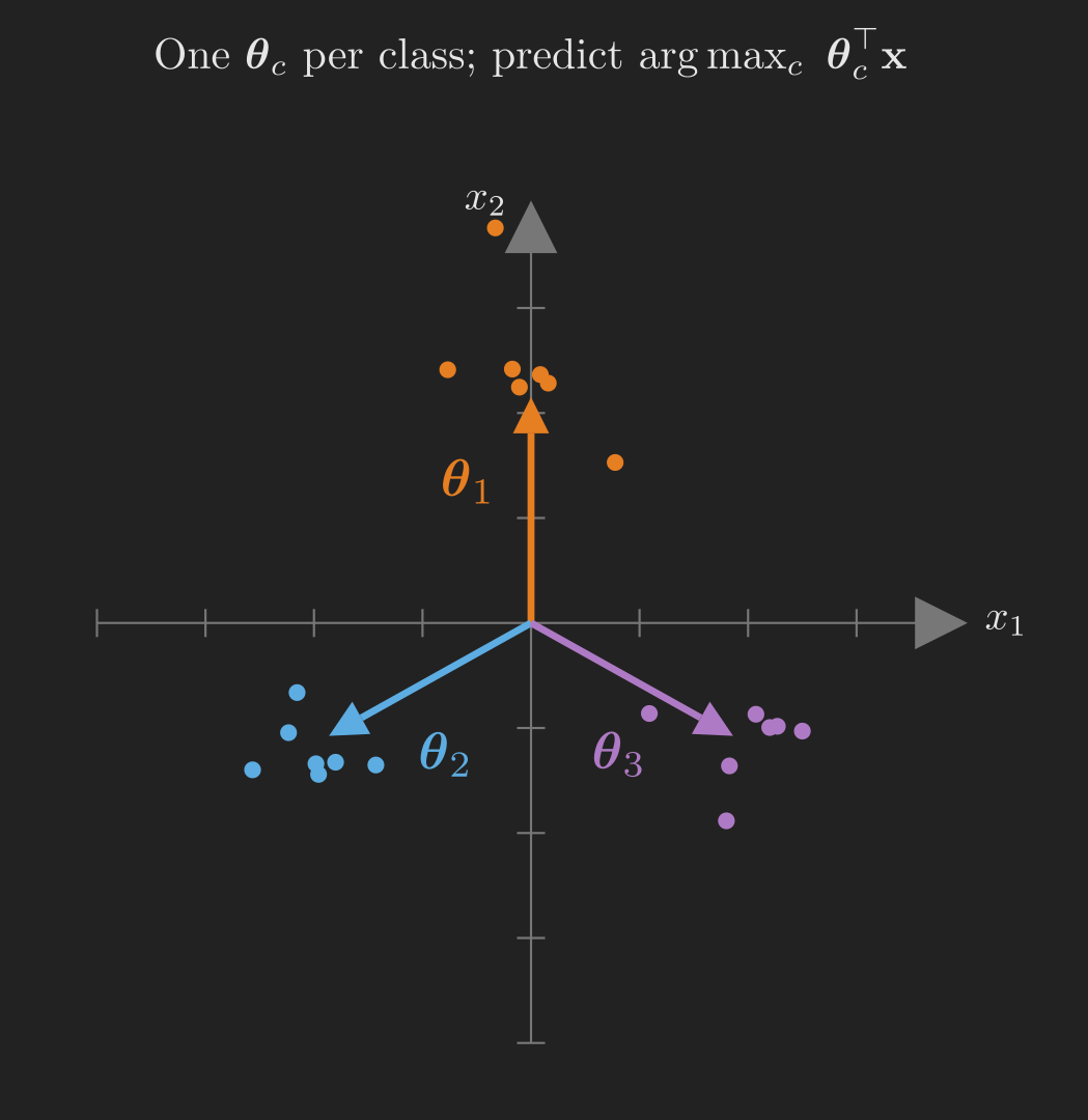
Concretely, given an input \(\vb{x}\), we compute \(k\) scores \(\boldsymbol{\uptheta}_1^{\intercal}\vb{x}, \ldots, \boldsymbol{\uptheta}_k^{\intercal}\vb{x}\), each a real number, and predict the class with the largest score, \(\operatorname*{arg\,max}_{c}\, \boldsymbol{\uptheta}_c^{\intercal}\vb{x}\). Because a dot product is large when two vectors point in similar directions, each \(\boldsymbol{\uptheta}_c\) ends up pointing toward its own class’s cluster, so examples from class \(c\) score highest against \(\boldsymbol{\uptheta}_c\).

That gives us a decision, but not probabilities, and not a differentiable loss to train on. The scores \(\boldsymbol{\uptheta}_c^{\intercal}\vb{x}\) (called logits) are just real numbers: some negative, and they do not sum to \(1\). We need to turn a vector of logits into a probability distribution.

From logits to probabilities: the softmax function

A probability distribution over \(k\) classes needs two things: every entry non-negative, and the entries summing to \(1\). So we fix the logits in two moves.

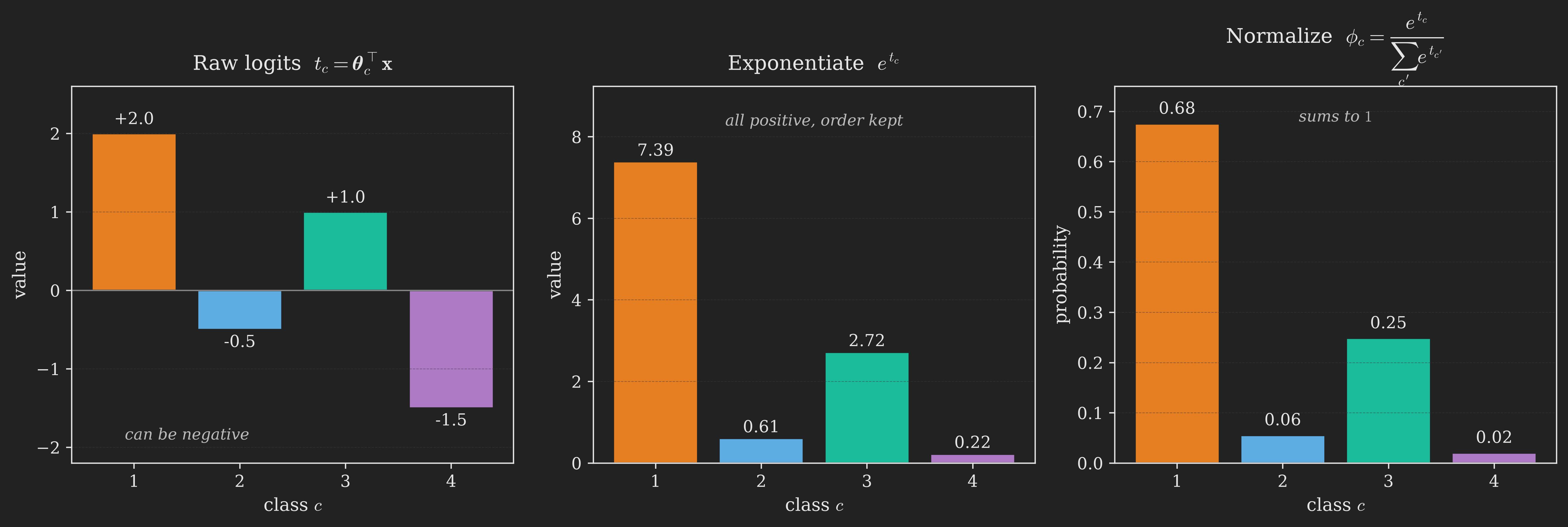
• Move 1: make everything positive, keeping the order. Exponentiate each logit. The function \(e^{t}\) sends any real number to a positive one, and it is increasing, so it preserves which logit was biggest. (Other tricks, like adding a constant or taking absolute values, either fail to guarantee positivity or scramble the order; exponentiating does both jobs at once.)
• Move 2: make them sum to \(1\). Divide each exponentiated value by their total.

Those two moves are the softmax function. Figure 4 shows them acting on four example logits.

Figure 4: The softmax function in two moves. Left: four raw logits \(t_c = \boldsymbol{\uptheta}_c^{\intercal}\vb{x}\), which can be negative and do not sum to anything in particular. Middle: exponentiating makes them all positive while preserving their order (the largest logit is still largest). Right: dividing by their sum yields a probability distribution over the four classes. The biggest logit gets the biggest probability.

Written out, with logits \(\left(t_1, \ldots, t_k\right)\),

\[ \operatorname{softmax}\left(t_1, \ldots, t_k\right) = \begin{pmatrix} \dfrac{\exp\left(t_1\right)}{\sum_{c'=1}^{k}\exp\left(t_{c'}\right)} \\[2ex] \vdots \\[1ex] \dfrac{\exp\left(t_k\right)}{\sum_{c'=1}^{k}\exp\left(t_{c'}\right)} \end{pmatrix}. \tag{4}\]

The name is apt: softmax is a smooth, differentiable stand-in for the (non-differentiable) \(\operatorname*{arg\,max}\). It does not just report the winner; it reports a soft, probabilistic vote that leans hardest toward the largest logit. That smoothness is exactly what lets us train it by gradient descent.

Setting the logits to our class scores, \(t_c = \boldsymbol{\uptheta}_c^{\intercal}\vb{x}\), gives the softmax regression model. The probability the model assigns to class \(c\) is

\[ \mathrm{P}\left(y = c \mid \vb{x}; \boldsymbol{\uptheta}\right) = \phi_c = \frac{\exp\left(t_c\right)}{\sum_{c'=1}^{k}\exp\left(t_{c'}\right)} = \frac{\exp\left(\boldsymbol{\uptheta}_c^{\intercal}\vb{x}\right)}{\sum_{c'=1}^{k}\exp\left(\boldsymbol{\uptheta}_{c'}^{\intercal}\vb{x}\right)}. \tag{5}\]

This is the multi-class GLM the zoo promised; it is what you get by choosing the categorical distribution in step 1 of the recipe. (Logistic regression is the \(k = 2\) special case: with two classes, Equation 5 collapses back to a single sigmoid.)

Training softmax regression: the cross-entropy loss

To train, we do what we always do: maximize the likelihood of the data, equivalently minimize the negative log-likelihood. For a single example \(\left(\vb{x}, y\right)\), the negative log-likelihood is the negative log of the probability Equation 5 assigns to the true class \(y\). This quantity is important enough to have its own name, the cross-entropy loss:

\[ \ell_{\text{ce}}\left(\left(t_1, \ldots, t_k\right), y\right) = -\log\left(\frac{\exp\left(t_y\right)}{\sum_{c'=1}^{k}\exp\left(t_{c'}\right)}\right). \tag{6}\]

Summing over all \(n\) training examples gives the total loss to minimize,

\[ \ell\left(\boldsymbol{\uptheta}\right) = \sum_{i=1}^{n} \ell_{\text{ce}}\left(\left(\boldsymbol{\uptheta}_1^{\intercal}\vb{x}_i, \ldots, \boldsymbol{\uptheta}_k^{\intercal}\vb{x}_i\right), y_i\right). \tag{7}\]

To run gradient descent we need the gradient of \(\ell\). It turns out to have a strikingly clean form, and the cleanliness is worth seeing.

NoteOptional deeper dive: deriving the cross-entropy gradient

Start with the loss for one example as a function of the logits \(\vb{t} = \left(t_1, \ldots, t_k\right)\). Using \(\log\left(a / b\right) = \log a - \log b\), rewrite Equation 6 as

\[ \ell_{\text{ce}}\left(\vb{t}, y\right) = -t_y + \log\left(\sum_{c'=1}^{k}\exp\left(t_{c'}\right)\right). \]

Differentiate with respect to one logit \(t_c\). The first term contributes \(-1\) only when \(c\) is the true class \(y\), i.e. \(-\mathbf{1}\left\{y = c\right\}\), where \(\mathbf{1}\left\{\cdot\right\}\) is the indicator function (\(1\) if its condition holds, \(0\) otherwise). The second term, by the chain rule, contributes \(\exp\left(t_c\right) / \sum_{c'}\exp\left(t_{c'}\right)\), which is exactly \(\phi_c\). Therefore

\[ \pdv{\ell_{\text{ce}}\left(\vb{t}, y\right)}{t_c} = \phi_c - \mathbf{1}\left\{y = c\right\}. \tag{8}\]

Now push through to the parameters. Since \(t_c = \boldsymbol{\uptheta}_c^{\intercal}\vb{x}\), we have \(\pdv{t_c}{\boldsymbol{\uptheta}_c} = \vb{x}\), and \(t_{c'}\) for \(c' \neq c\) does not depend on \(\boldsymbol{\uptheta}_c\). By the chain rule,

\[ \pdv{\ell_{\text{ce}}}{\boldsymbol{\uptheta}_c} = \pdv{\ell_{\text{ce}}}{t_c}\cdot\pdv{t_c}{\boldsymbol{\uptheta}_c} = \left(\phi_c - \mathbf{1}\left\{y = c\right\}\right)\vb{x}. \]

The gradient with respect to logit \(t_c\) is beautifully simple:

\[ \pdv{\ell_{\text{ce}}\left(\vb{t}, y\right)}{t_c} = \phi_c - \mathbf{1}\left\{y = c\right\}, \tag{9}\]

which reads, in words, “predicted probability of class \(c\), minus \(1\) if \(c\) is the true class.” In compact vector form it is even tidier: \(\pdv{\ell_{\text{ce}}}{\vb{t}} = \boldsymbol{\upphi} - \vb{e}_y\), where \(\boldsymbol{\upphi}\) is the vector of predicted probabilities and \(\vb{e}_y\) is the one-hot vector with a \(1\) in the true class’s slot. Propagating through to the parameters, the gradient of the total loss with respect to class \(c\)’s parameters is

\[ \pdv{\ell\left(\boldsymbol{\uptheta}\right)}{\boldsymbol{\uptheta}_c} = \sum_{i=1}^{n}\left(\phi_{c,i} - \mathbf{1}\left\{y_i = c\right\}\right)\vb{x}_i, \tag{10}\]

where \(\phi_{c,i}\) is the probability the model assigns to class \(c\) for example \(i\). Look closely at Equation 10 and compare it to the universal GLM update Equation 3: it is the same “prediction minus target, times input” shape, now written per class, with the target being \(1\) for the correct class and \(0\) for the rest. The pattern that ran through every earlier algorithm runs through this one too. With this gradient, plain (stochastic) gradient descent trains the model.

Let us place softmax on the map before closing.

flowchart TB
    A["<b>1. A New Data Type</b>"]
    B["<b>2. Two Clues</b>"]
    C["<b>3. The Exponential Family</b>"]
    D["<b>4. Two Gifts</b>"]
    E["<b>5. The GLM Recipe</b>"]
    F["<b>6. Turning the Crank</b>"]
    G["<b>7. Three Parameters</b>"]
    H["<b>8. The Zoo of GLMs</b>"]
    I["<b>9. Softmax Regression</b><br/>Many classes, one loss"]
    J["<b>10. Wrapping Up</b>"]
    A --> B --> C --> D --> E --> F --> G --> H --> I --> J

    style I fill:#c0392b,color:#fff,stroke:#fff

Wrapping Up

We started with a coffee shop and a nagging worry: every new kind of output seemed to demand a new algorithm, derived painfully from scratch. We end with a single recipe that dissolves the worry.

The key realization is that linear regression and logistic regression were never two separate inventions. They are two turns of one crank. That crank has three steps: (1) pick the exponential-family distribution matching your data type, (2) predict its mean, and (3) make the natural parameter \(\boldsymbol{\uptheta}^{\intercal}\vb{x}\). The exponential family is what makes the crank turn smoothly, because writing any distribution in the form \(p\left(y; \eta\right) = b\left(y\right)\exp\left(\eta \, T\left(y\right) - a\left(\eta\right)\right)\) hands you a convex loss (Gift 1) and its mean as a simple derivative \(a'\left(\eta\right)\) (Gift 2).

From that one recipe, everything followed. The sigmoid stopped being arbitrary: it is precisely the Bernoulli’s canonical response function, forced on us the moment we say “binary.” The mysteriously shared update rule stopped being a coincidence: it is a theorem, a direct consequence of Gift 2, that “target minus prediction, times input” is the log-likelihood gradient for every GLM. And the coffee shop’s counting problem, which stumped both of our old tools, was solved almost for free by choosing the Poisson and reading off \(h_{\boldsymbol{\uptheta}}\left(\vb{x}\right) = e^{\boldsymbol{\uptheta}^{\intercal}\vb{x}}\). We even built softmax regression for many classes at once, and watched the same “prediction minus target” gradient reappear.

If you keep just one image, keep the three-parameter line: the global model parameters \(\boldsymbol{\uptheta}\) dot with an input to make the per-example natural parameter \(\eta\), and the canonical response function \(g\) turns \(\eta\) into the mean, which is the prediction.

flowchart TB
    A["<b>1. A New Data Type</b>"]
    B["<b>2. Two Clues</b>"]
    C["<b>3. The Exponential Family</b>"]
    D["<b>4. Two Gifts</b>"]
    E["<b>5. The GLM Recipe</b>"]
    F["<b>6. Turning the Crank</b>"]
    G["<b>7. Three Parameters</b>"]
    H["<b>8. The Zoo of GLMs</b>"]
    I["<b>9. Softmax Regression</b>"]
    J["<b>10. Wrapping Up</b><br/>One recipe, many models"]
    A --> B --> C --> D --> E --> F --> G --> H --> I --> J

    style J fill:#b9770e,color:#fff,stroke:#fff

Where does this thread lead next? Look again at assumption 3, the one we called a “design choice”: \(\eta = \boldsymbol{\uptheta}^{\intercal}\vb{x}\). We chose to make the natural parameter linear in the features. Loosen that choice, let \(\eta\) be produced by something richer than a single linear layer, stack several such transformations, and you have taken the first step toward neural networks. And the cross-entropy loss Equation 6, with its clean \(\boldsymbol{\upphi} - \vb{e}_y\) gradient, is exactly the loss that sits at the output of nearly every classification network trained today; that same gradient will come back when we study backpropagation. The recipe you learned here is not a dead end; it is the base camp.

Acknowledgment

This post is based on the sixth lecture of the Stanford CS229 Machine Learning course (Summer 2019), delivered by Anand Avati (Stanford Online, Anand Avati, 2019), and on the accompanying course notes by Andrew Ng (Ng & Ma, 2023). The generalized linear model framework itself is developed in full by McCullagh & Nelder (1989), and complementary treatments of the exponential family appear in Bishop (2006) and Hastie et al. (2009).

References

Bishop, C. M. (2006). Pattern Recognition and Machine Learning. Springer.

Hastie, T., Tibshirani, R., Friedman, J., et al. (2009). The Elements of Statistical Learning: Data Mining, Inference, and Prediction. Springer series in statistics New-York.

McCullagh, P., & Nelder, J. A. (1989). Generalized Linear Models (2nd ed.). Chapman; Hall/CRC.

Ng, A., & Ma, T. (2023). CS229 Lecture Notes. Stanford University; https://cs229.stanford.edu/main_notes.pdf.

Stanford Online, Anand Avati. (2019). Stanford CS229: Machine Learning Course | Summer 2019. Stanford University; https://youtube.com/playlist?list=PLoROMvodv4rNH7qL6-efu_q2_bPuy0adh.