%%{init: {'theme':'dark', 'themeVariables': { 'primaryColor': '#375a7f', 'primaryTextColor': '#fff', 'primaryBorderColor': '#6c757d', 'lineColor': '#adb5bd', 'secondaryColor': '#444', 'tertiaryColor': '#222'}}}%%
flowchart TD
 subgraph Client["Client"]
 EXT[Chrome Extension<br/>popup.html / popup.js]
 end

 subgraph External["External API"]
 YT[YouTube Data API v3]
 end

 subgraph AWS["AWS Serving Layer"]
 ALB[Application<br/>Load Balancer]
 ASG[Auto Scaling Group<br/>EC2 × 2-3]
 DOCK[Docker Container<br/>FastAPI + LightGBM]
 ALB --> ASG
 ASG --> DOCK
 end

 subgraph MLOps["MLOps Layer"]
 MLF[MLflow Registry<br/>on DagsHub]
 S3[(S3:<br/>raw data + DVC remote)]
 ECR[(ECR:<br/>Docker image)]
 end

 EXT -- "fetch comments" --> YT
 YT -- "comments + metadata" --> EXT
 EXT -- "POST /predict<br/>/generate_chart<br/>/generate_wordcloud<br/>/generate_trend_graph" --> ALB
 DOCK -- "load model<br/>at startup" --> MLF
 DOCK -- "pull image" --> ECR
 MLF -.-> S3
YouTube Comment Intelligence
Machine Learning
NLP
MLOps
An end-to-end MLOps system that delivers real-time sentiment analysis of YouTube comments through a Chrome extension, backed by a FastAPI service deployed on AWS.
1 TL;DR
YouTube Comment Intelligence is a production-grade machine learning system that gives content creators actionable insight into the conversations happening under their videos. Open the Chrome extension on any YouTube video and it pulls the comments through the YouTube Data API, sends them to a FastAPI service running behind an Application Load Balancer on AWS, and returns a full analytical view: sentiment distribution, a word cloud, a monthly sentiment trend, the top-25 comments with predicted labels, and headline metrics like the number of unique commenters and an average sentiment score.
Underneath the product is a complete MLOps loop: data versioned with DVC and stored on S3, experiments tracked on MLflow (hosted on DagsHub), models promoted through a staging → production workflow in the MLflow Model Registry, the whole training pipeline reproducible via a single dvc repro, and a GitHub Actions workflow that on every push retrains, tests, builds a Docker image, pushes to ECR, and triggers a CodeDeploy rolling deployment onto an EC2 Auto Scaling Group fronted by a load balancer.
The sentiment model itself is a LightGBM classifier trained on Reddit comments (Twitter data was rejected during EDA for being too politically skewed) with bag-of-words bigrams and class_weight="balanced" to handle class imbalance, a choice that emerged from five structured experiments covering feature engineering, max_features tuning, resampling strategies, model comparison, and extensive hyperparameter search with Optuna.
This post walks through the system top-down, architecture first, then each layer in detail.
2 System Architecture
2.1 High-Level View
At the highest level, the system has three tiers: a client (the Chrome extension running in the user’s browser), a serving layer (a FastAPI application running in a Docker container on EC2, fronted by an Application Load Balancer), and an MLOps layer (DVC pipeline, MLflow Model Registry, S3 artifact storage, GitHub Actions CI/CD).
The client never talks to the model directly. It always goes through the load balancer, which spreads traffic across the healthy EC2 instances in the Auto Scaling Group. Each instance runs the same Docker image (pulled from ECR at deployment time), which in turn loads the current “Production” model from the MLflow Registry during FastAPI’s startup event. This means rolling out a new model is just a matter of promoting a new version in the registry and restarting the containers. No code changes required.
2.2 Request Flow: What Happens When You Click the Extension
The extension exposes five backend endpoints. The most interesting is the main flow for the “full analysis” view:
%%{init: {'theme':'dark', 'themeVariables': { 'primaryColor': '#375a7f', 'primaryTextColor': '#fff', 'primaryBorderColor': '#6c757d', 'lineColor': '#adb5bd', 'actorBkg':'#375a7f', 'actorTextColor':'#fff', 'signalColor':'#adb5bd', 'signalTextColor':'#fff'}}}%%
sequenceDiagram
 autonumber
 participant U as User
 participant X as Extension
 participant Y as YouTube Data API
 participant L as ALB
 participant F as FastAPI (EC2)
 participant M as MLflow Registry

 U->>X: Clicks extension icon on a YouTube video
 X->>X: Validate URL, extract videoId
 X->>Y: GET commentThreads?videoId=...
 Y-->>X: comments + authors + timestamps
 X->>L: POST /predict_with_timestamps
 L->>F: Forward to healthy instance
 F->>F: Preprocess → vectorize → predict
 F-->>X: [{comment, sentiment, timestamp}, …]
 par Parallel enrichment calls
 X->>L: POST /generate_chart (sentiment counts)
 L->>F: Forward
 F-->>X: pie chart PNG
 and
 X->>L: POST /generate_wordcloud (comments)
 L->>F: Forward
 F-->>X: word cloud PNG
 and
 X->>L: POST /generate_trend_graph (timestamped labels)
 L->>F: Forward
 F-->>X: monthly trend PNG
 end
 X->>U: Render dashboard in popup
 Note over F,M: Model & vectorizer<br/>loaded once at startup
The parallelism in steps 8-10 matters for latency, the extension issues the three “generation” requests concurrently rather than serially, so the total wall-clock time the user waits on is roughly the slowest of the three chart calls plus the sentiment inference, not their sum.
2.3 The MLOps Loop
The training-and-deployment side is a closed loop. A push to main can, and usually does, propagate all the way to a new model in production:
%%{init: {'theme':'dark', 'themeVariables': { 'primaryColor': '#375a7f', 'primaryTextColor': '#fff', 'primaryBorderColor': '#6c757d', 'lineColor': '#adb5bd'}}}%%
flowchart TB
 DEV[git push] --> GHA[GitHub Actions<br/>ci-cd.yaml]

 subgraph CI["Continuous Integration"]
 GHA --> DVC[dvc repro<br/>6-stage pipeline]
 DVC --> REG[Register model → Staging]
 REG --> T1[Model loading test]
 T1 --> T2[Model signature test]
 T2 --> T3[Performance test<br/>≥ 0.75 thresholds]
 T3 --> PROMO[Promote → Production<br/>archive old]
 PROMO --> API[FastAPI endpoint tests]
 end

 subgraph CD["Continuous Delivery"]
 API --> BUILD[Build Docker image]
 BUILD --> PUSH[Push to ECR]
 PUSH --> ZIP[Zip appspec.yml +<br/>deploy scripts → S3]
 ZIP --> CD_TRIG[Trigger CodeDeploy]
 CD_TRIG --> ROLL[Rolling deploy<br/>OneAtATime across ASG]
 end

 ROLL --> PROD[Production]

 style PROMO fill:#00bc8c,stroke:#fff,color:#fff
 style PROD fill:#00bc8c,stroke:#fff,color:#fff
 style T3 fill:#e74c3c,stroke:#fff,color:#fff
The two gates that matter most are the performance test (a model that falls below 0.75 on accuracy / precision / recall / F1 on a held-out slice never makes it out of Staging) and the rolling deployment (CodeDeploy’s OneAtATime config, combined with the ALB health checks, means a broken build can’t take down the whole fleet).
3 Problem Framing
3.1 Business Context
Imagine an influencer management company trying to expand its roster but working with a limited marketing budget. Paid acquisition is out. The alternative is to give influencers something genuinely useful, a tool that solves a real pain point so well that they come to you.
The pain point is obvious once you look at any sufficiently popular channel: comment sections with tens of thousands of entries that no human can read, let alone analyze. Creators want to know things like what is the overall sentiment on this video?, what are people actually talking about?, and is the conversation getting more or less positive over time?, and they currently have no good way to answer any of them.
3.2 Product Requirements
The extension was scoped around four capabilities:
- Real-time sentiment classification of every comment as positive, neutral, or negative, with visual distribution (pie chart) and drill-downs into individual comments.
- Word cloud over all comments so themes jump out at a glance.
- Sentiment trend over time (monthly line chart) so creators can see how audience mood evolved.
- Headline metrics: total comments, unique commenters, average words per comment, and an average sentiment score on a −10 to +10 scale.
3.3 Technical Challenges
Before writing a line of code it was worth cataloguing what was going to be hard:
- No labelled YouTube data. The YouTube Data API returns comments but no sentiment labels. The nearest available labelled corpus was a Kaggle dataset containing both Reddit and Twitter comments, the Twitter subset turned out to be heavily political during EDA, so the model was trained on the Reddit subset only, which generalized better.
- No universally representative corpus. YouTube content is extraordinarily heterogeneous (cooking, politics, gaming, music, and so on). One model cannot be equally strong across all of them. This is accepted as a known limitation.
- Multilingual and code-switched comments, including English-scripted Hindi and similar transliterations. Out of scope for v1.
- Spam, bots, sarcasm, slang, emoji, evolving Gen-Z vocabulary: all real sources of noise that bias or mislabel training signal.
- Latency. The extension must feel responsive. Hundreds of comments need to be classified and visualized in a few seconds at most.
- Privacy / compliance. The source of training data matters if the system is ever commercialized; using licensed Kaggle data is a deliberate choice.
4 The Sentiment Model
This is the heart of the system. The goal of this section isn’t to enumerate every experiment, it’s to show the reasoning chain that led from a 65%-accuracy baseline to the LightGBM model in production.
4.1 Data
- Source: Kaggle “Twitter and Reddit Sentimental Analysis Dataset”, only the Reddit subset.
- Size: ~37,249 comments after light cleaning.
- Labels:
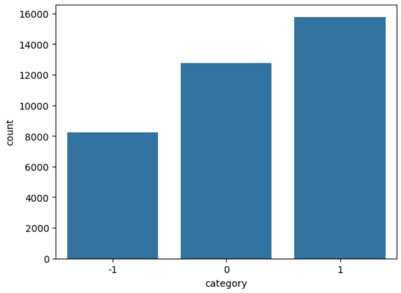
-1(negative),0(neutral),+1(positive). - Class distribution: 43% positive, 35% neutral, 22% negative. This is a moderate imbalance that, as we’ll see, drives most of the early model’s failure modes.
4.2 Exploratory Data Analysis
EDA and preprocessing were done in tight cycles: clean a bit, look at distributions, adjust the cleaning, look again. The full EDA notebook lives here.
4.2.1 Cleaning Steps That Actually Fired
- Explicit NaNs: 100 out of 37,249 comments, dropped (all were labelled neutral).
- Whitespace-only comments: 6, dropped.
- Duplicates: 350, dropped.
- Leading/trailing whitespace: 32,266 comments, stripped.
- URLs: none found by regex match; no-op.
- Newlines and tabs: replaced with a single space.
- Non-English special characters: removed via regex.
- Punctuation: already absent from the source.
4.2.2 Class Imbalance
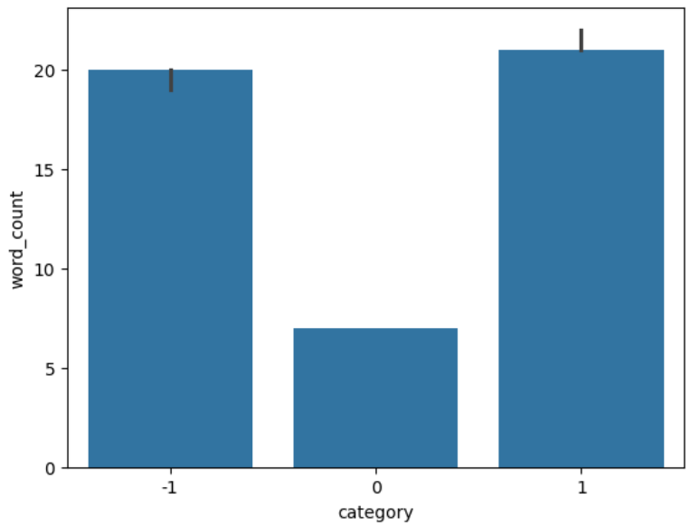
4.2.3 Length-Based Features
Several columns were engineered to probe whether comment length carried any sentiment signal.
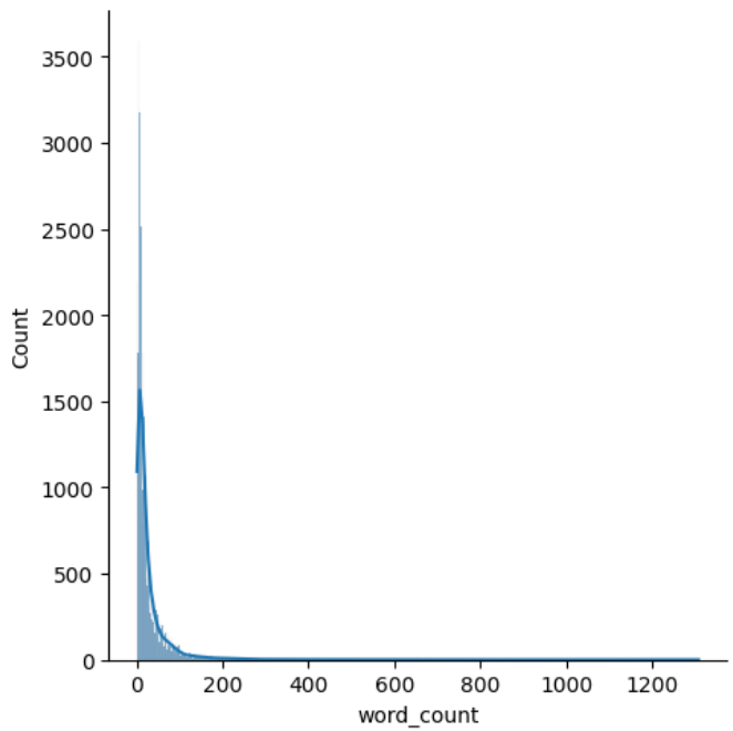
The word_count distribution is heavily right-skewed, most comments are short, with a long thin tail of unusually long ones.
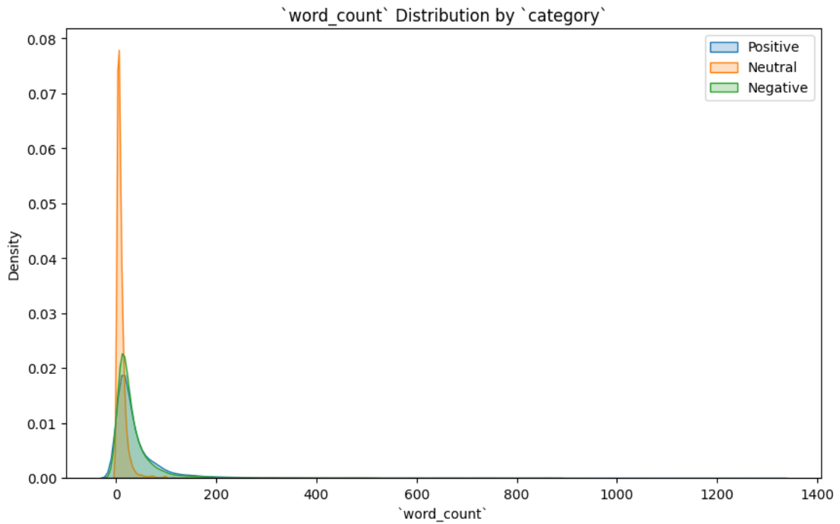
Broken down by sentiment, neutral comments are noticeably shorter and more concentrated around small word counts. Positive and negative comments have wider spreads and behave similarly to each other.
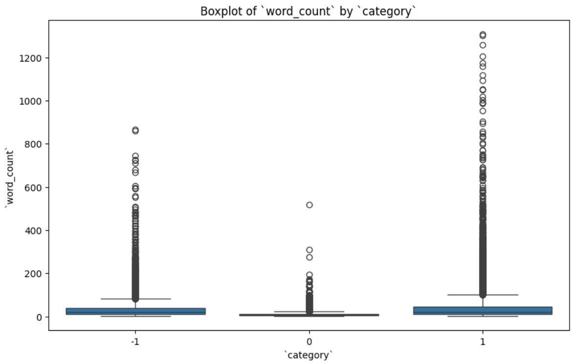
The box plot confirms that neutral comments have the lowest median and tightest IQR; positive comments sit slightly above negative ones in median but both have long upper tails.
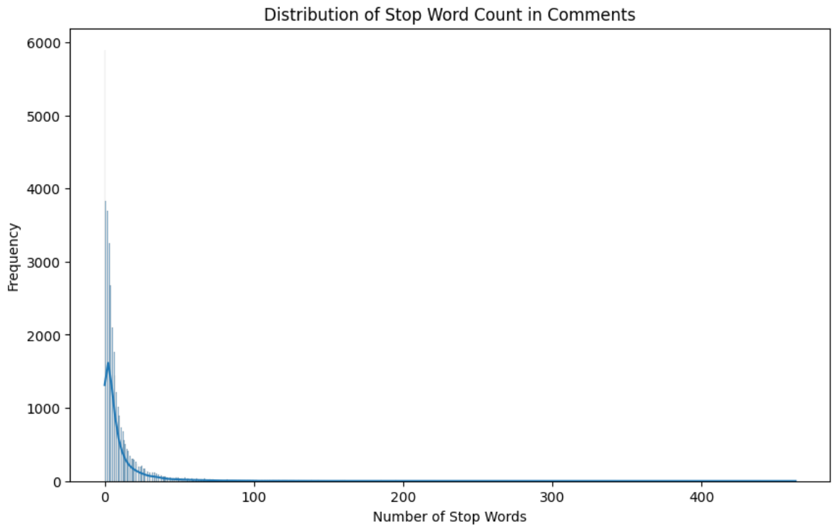
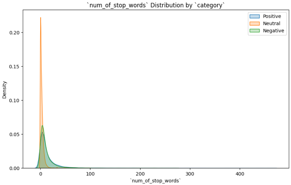
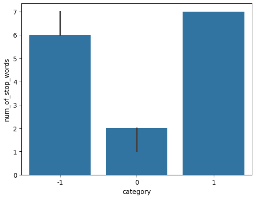
4.2.4 Stop Word Analysis
A num_of_stop_words feature was built using NLTK. Its distributions mirrored word_count almost exactly (right skew, neutral concentrated at the low end), which is unsurprising.
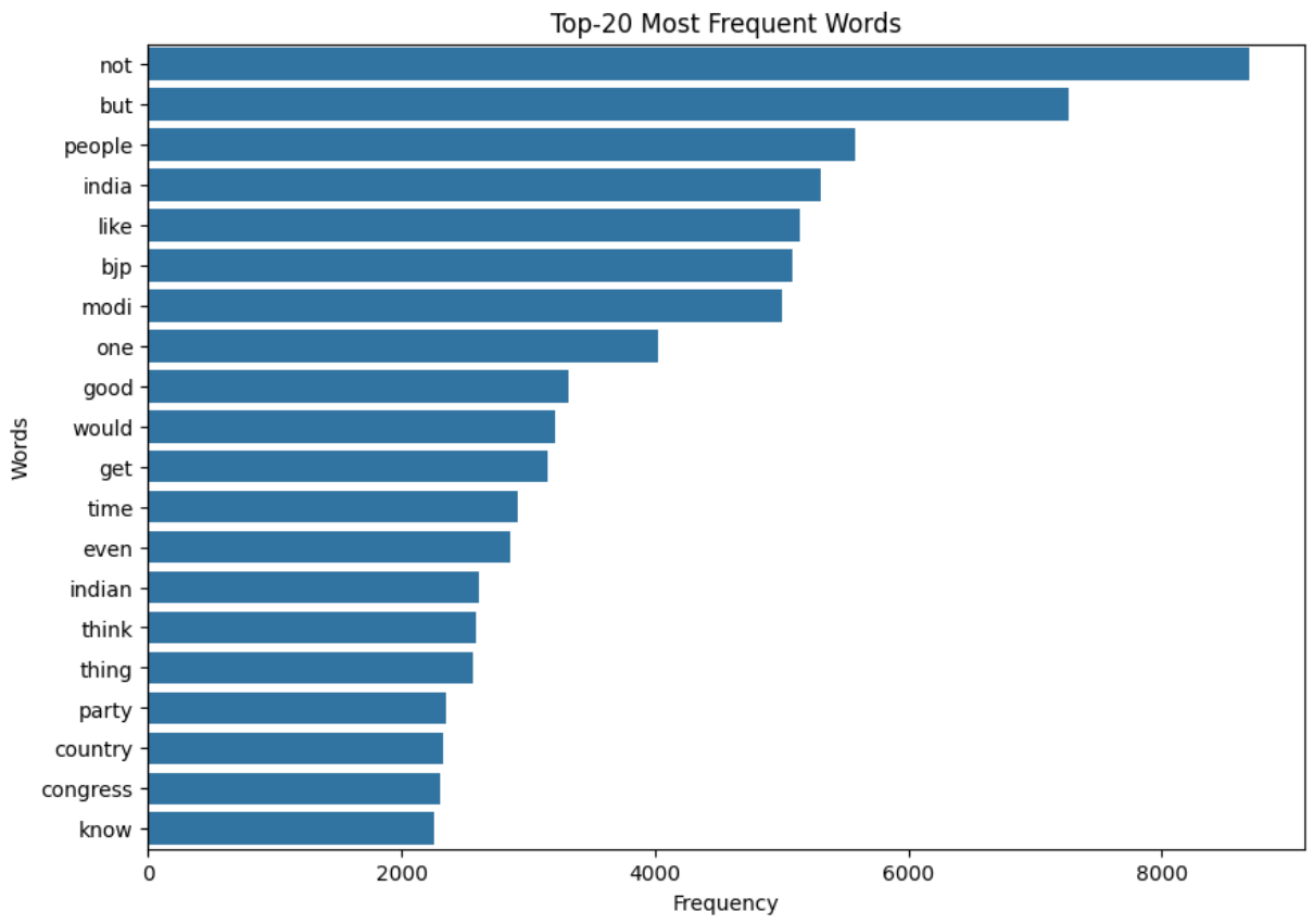
The interesting finding was in the top-25 stop words:
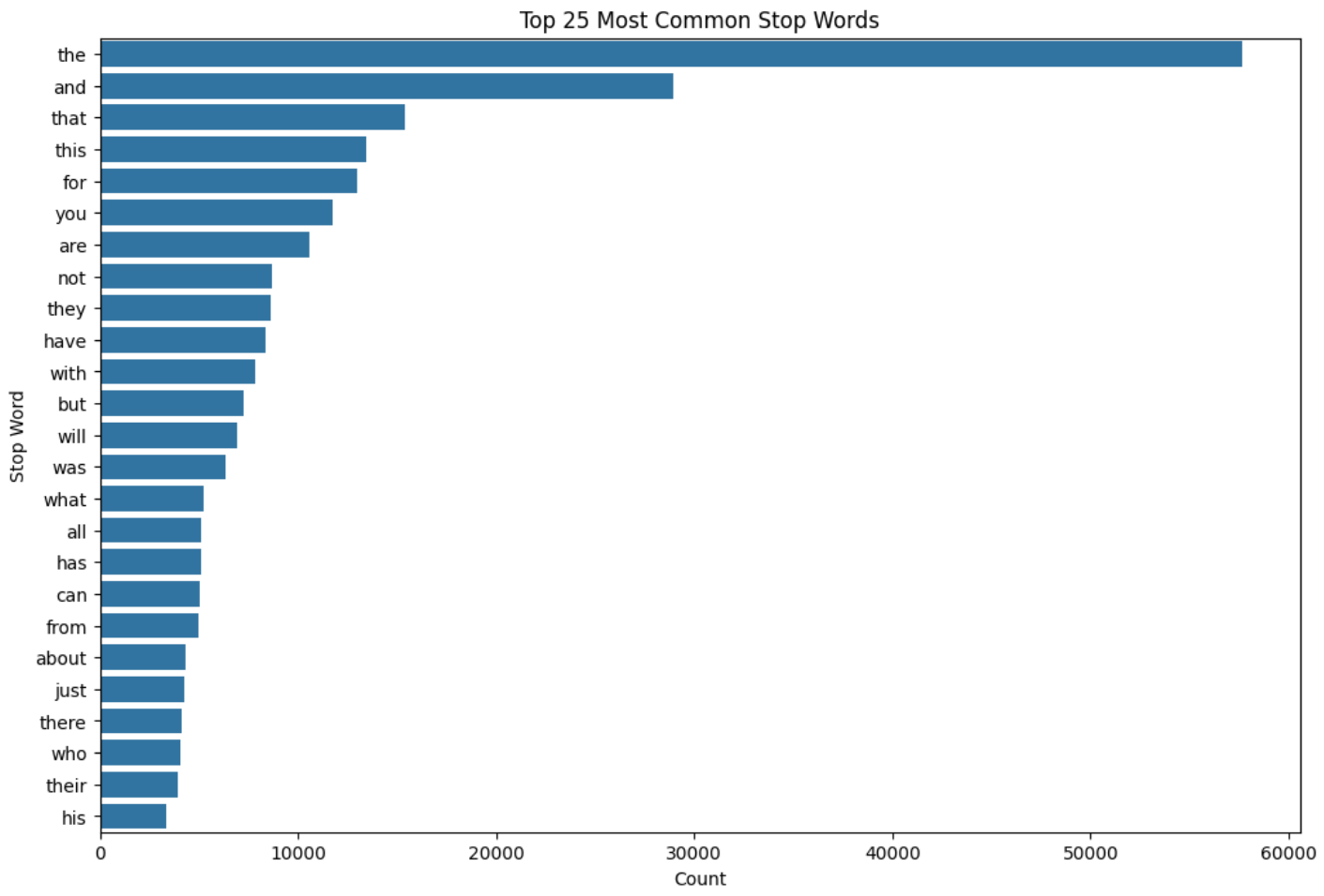
The word not ranks extremely high. not, along with but, however, no, and yet, can invert the sentiment of an entire sentence. The stop word removal step was therefore configured to preserve these five words rather than using NLTK’s default list wholesale. This is a small but important decision. Stripping “not” would turn “this is not good” into “this is good” from the model’s point of view.
4.2.5 Character Counts
A num_chars feature was created. During this step the data revealed the presence of many non-English special characters, which were stripped via regex.
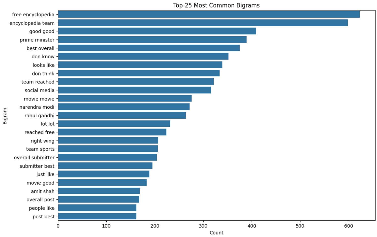
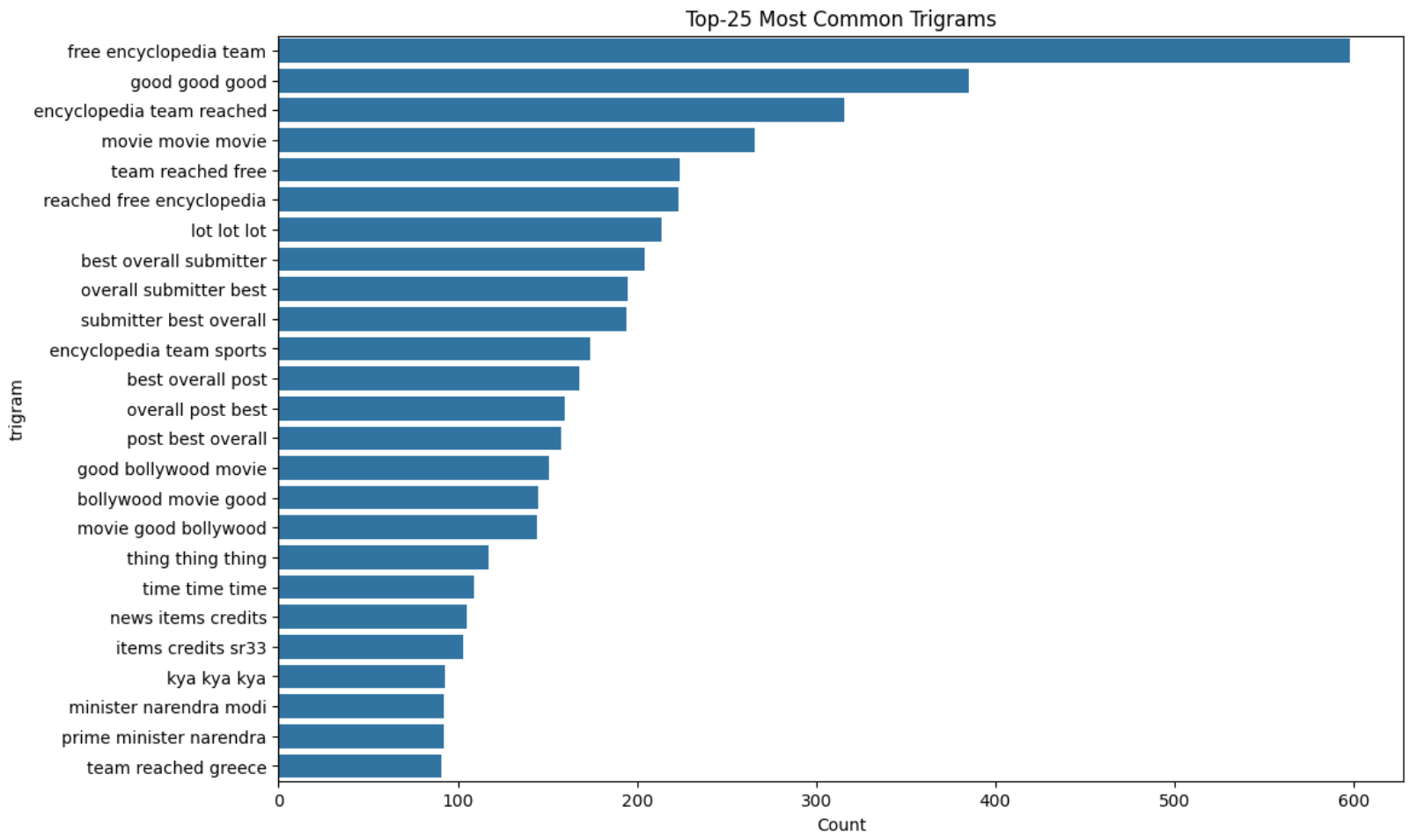
4.2.6 Bigrams and Trigrams
4.2.7 Lemmatization
All tokens were reduced to their root form with NLTK’s WordNetLemmatizer.
4.2.8 Word Clouds
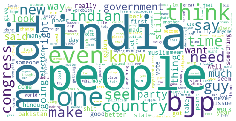
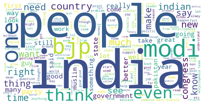
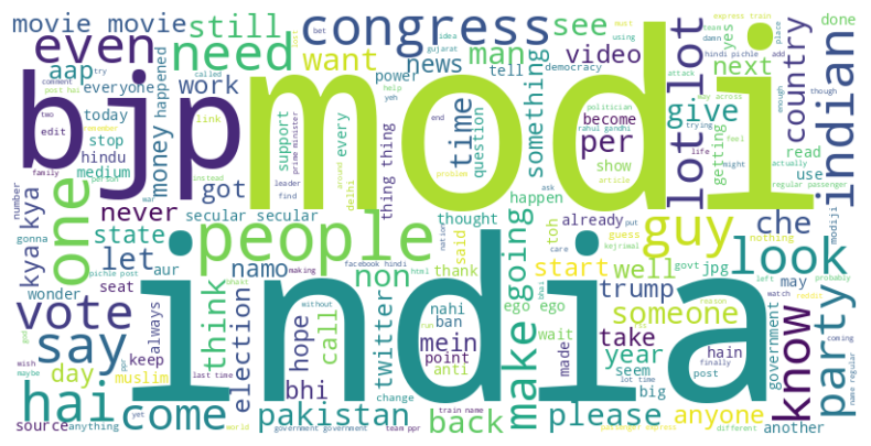
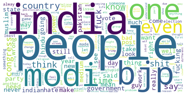
A somewhat uncomfortable observation: the dominant words are broadly similar across sentiment classes. That signals early that a bag-of-words model will need to rely on combinations (bigrams, contextual co-occurrence) rather than individual tokens to separate the classes.
4.2.9 Most Frequent Words
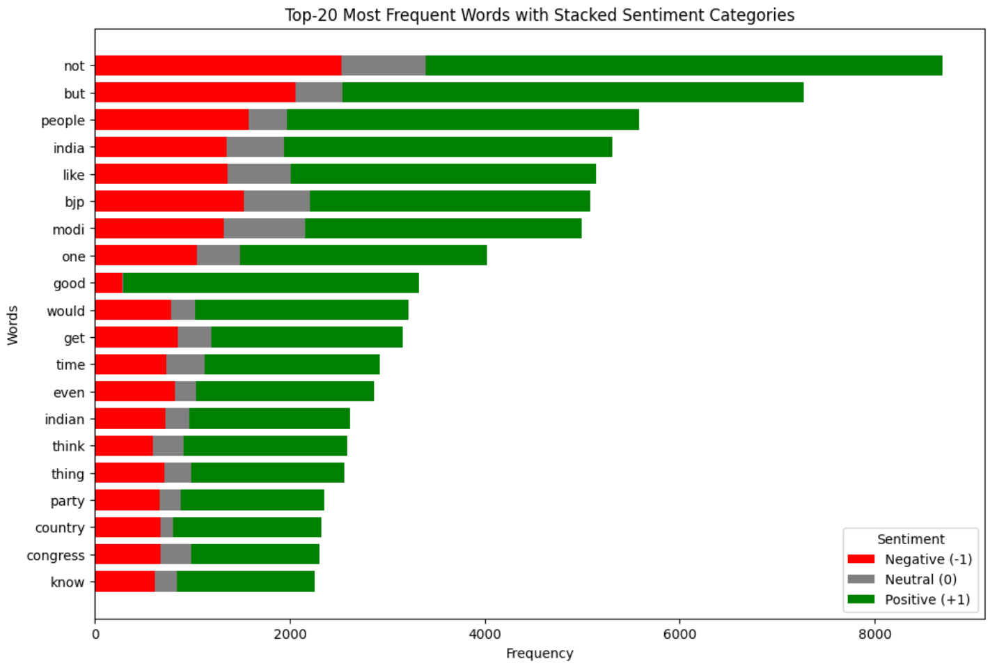
Same caveat as the word clouds: the lists look similar across sentiments, and the data leans political. Expect the model to transfer better to political content than, say, cooking tutorials.
4.3 Baseline: Random Forest + Bag of Words
The baseline was deliberately simple so subsequent experiments would have a clear reference point.
- Vectorizer:
CountVectorizer(unigrams). - Model:
RandomForestClassifierwith default-ish hyperparameters. - Experiment tracking: MLflow server hosted on DagsHub, logging metrics, the confusion matrix heatmap, the model, and the training data.
Best test accuracy: ~65%.
| Class | Precision | Recall | F1-score | Support |
|---|---|---|---|---|
| -1 (negative) | 1.00 | 0.02 | 0.03 | 1650 |
| 0 (neutral) | 0.66 | 0.85 | 0.74 | 2555 |
| +1 (positive) | 0.64 | 0.82 | 0.72 | 3154 |
| Accuracy | 0.65 | 7359 | ||
| Macro avg | 0.77 | 0.56 | 0.49 | 7359 |
| Weighted avg | 0.73 | 0.65 | 0.57 | 7359 |
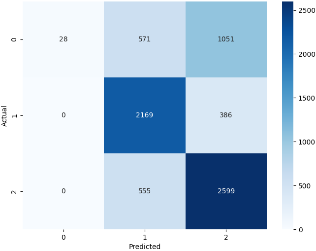
The failure is diagnostic. Recall on the negative class is ~0.02, the model classified just 28 out of 1,650 actual negatives correctly:
\[ \text{Recall (negative)} = \frac{28}{28 + 571 + 1051} = \frac{28}{1650} \approx 0.02 \]
But of the 28 it did flag as negative, every single one actually was, precision of 1.0:
\[ \text{Precision (negative)} = \frac{28}{28 + 0 + 0} = 1.0 \]
So the model isn’t “bad at negatives” per se, it’s refusing to predict negative almost entirely, defaulting to the majority classes. That’s the signature of class imbalance, and it dictates the direction of everything that follows. Baseline notebook.
4.4 Experiment Plan
Five structured experiments, each isolating one variable:
%%{init: {'theme':'dark', 'themeVariables': { 'primaryColor': '#375a7f', 'primaryTextColor': '#fff', 'primaryBorderColor': '#6c757d', 'lineColor': '#adb5bd'}}}%%
flowchart TD
 E1[Exp 1:<br/>BoW vs TF-IDF<br/>× n-gram range] --> E2[Exp 2:<br/>max_features<br/>sweep]
 E2 --> E3[Exp 3:<br/>Resampling<br/>strategy]
 E3 --> E4[Exp 4:<br/>Model family<br/>comparison]
 E4 --> E5[Exp 5:<br/>Fine HPT on<br/>top 4 models]
 E5 --> E6[Exp 6:<br/>Targeted LightGBM<br/>improvements]
4.4.1 Experiment 1: Feature Engineering
max_features fixed at 5,000. Swept vectorizer ∈ {BoW, TF-IDF} × n-gram ∈ {uni, bi, tri}.
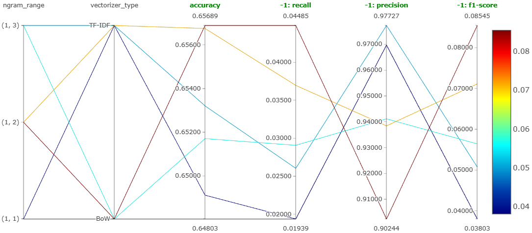
Winner: Bag-of-Words with bigrams. Notebook.
4.4.2 Experiment 2: max_features
Swept max_features from 1,000 to 10,000 in steps of 1,000 using BoW + bigrams.
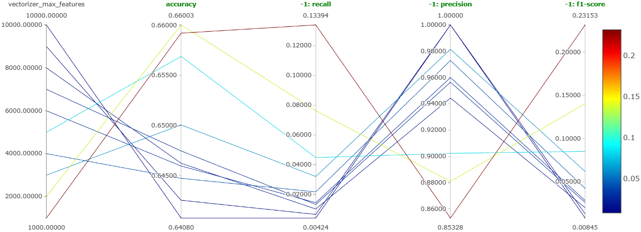
Winner: max_features = 1000. Lower values gave both higher overall accuracy and dramatically better recall on the negative class. This is a classic bias-variance win, narrower vocabulary, less overfitting on rare feature combinations. Notebook.
4.4.3 Experiment 3: Handling Class Imbalance
Candidates: undersampling, ADASYN, SMOTE, SMOTE+ENN, class weights in random forest.
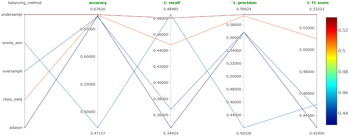
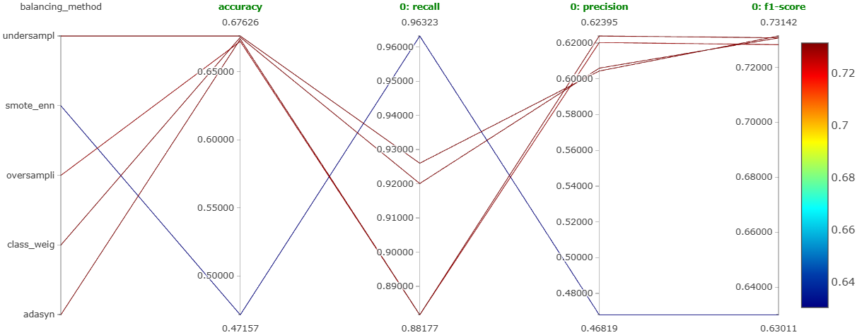
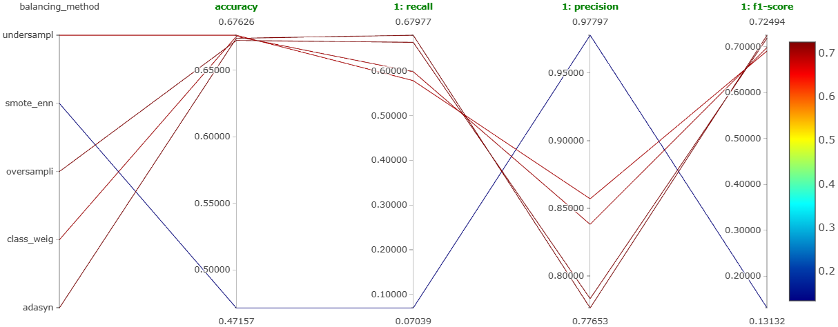
Winner: random undersampling, the most balanced performance across all three classes, not necessarily the highest on any single one. Notebook.
4.4.4 Experiment 4: Model Comparison
Seven models (XGBoost, LightGBM, random forest, SVM, logistic regression, KNN, naive Bayes), each with coarse Optuna HPT, each best version logged as a single MLflow run.
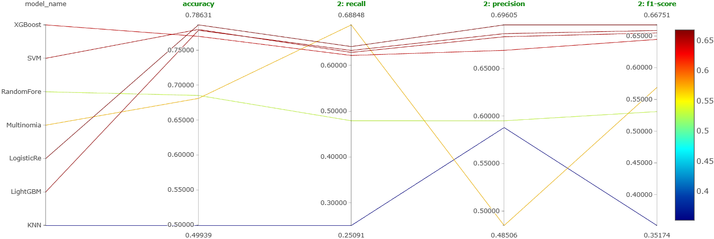
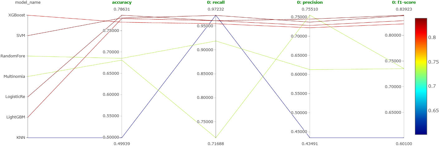
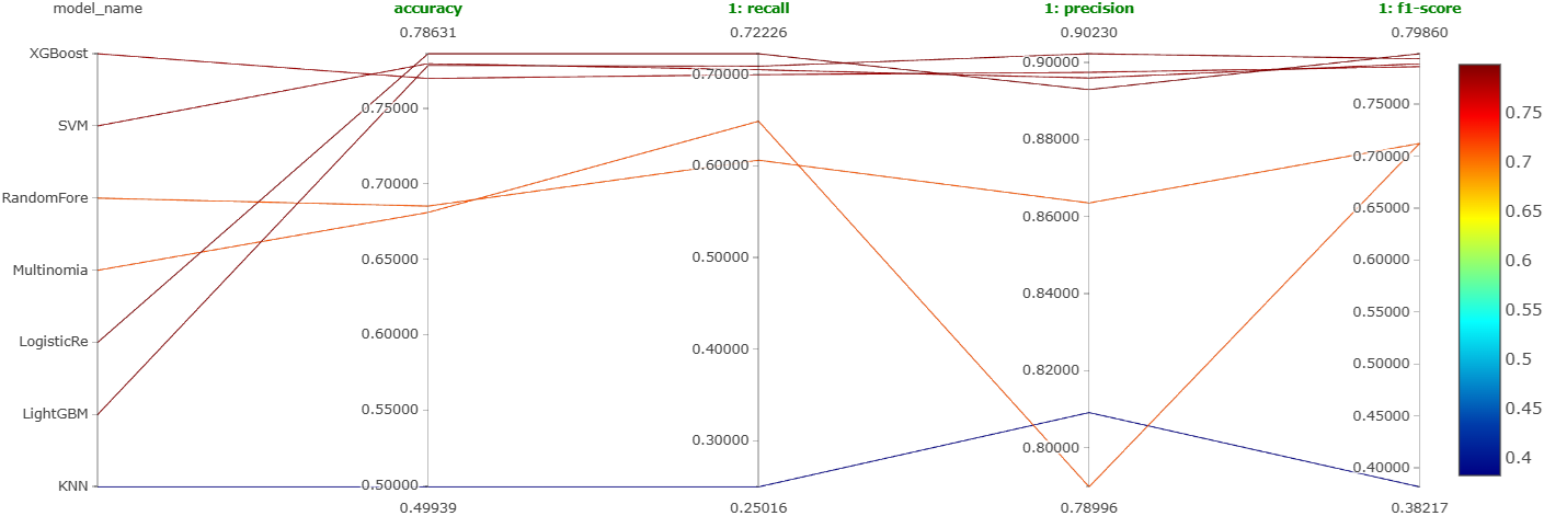
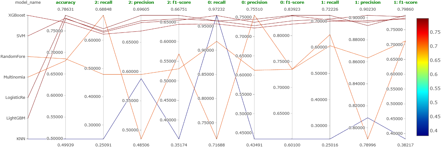
Four-way tie at the top: XGBoost, LightGBM, SVM, and logistic regression clustered tightly together with no clear winner. Notebooks: XGBoost, LightGBM, SVM, LogReg, KNN, Naive Bayes, Random Forest.
4.4.5 Experiment 5: Fine Hyperparameter Tuning
Extensive Optuna search on the four tied models.
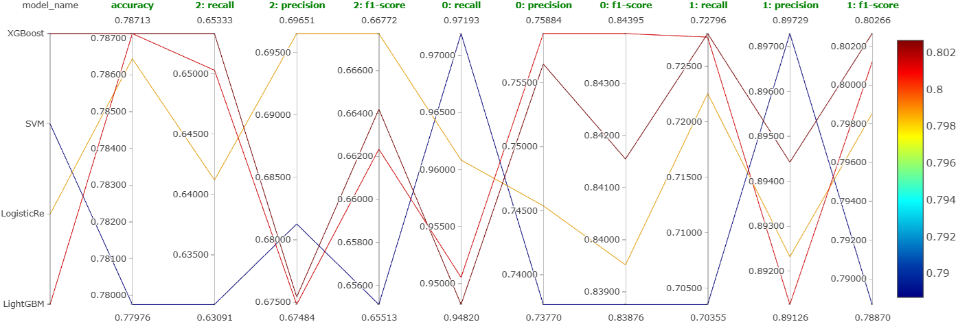
Still no clear winner after extensive tuning, accuracy stuck under 80%. LightGBM chosen for its combination of speed and the fact that ensemble tree methods tended to be more robust at the decision boundary between neutral and positive comments.
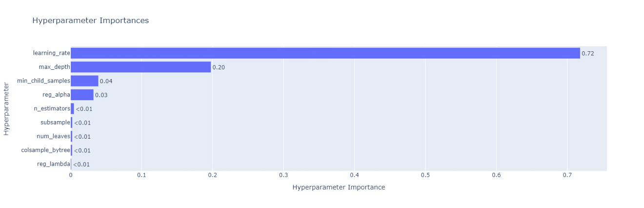
The top three hyperparameters by importance: learning_rate, max_depth, min_child_samples. Notebooks: LightGBM, XGBoost, SVM, LogReg.
4.5 Pushing LightGBM Further
Four targeted improvement attempts:
| Technique | Notebook | Verdict |
|---|---|---|
class_weight="balanced" |
18 | Chosen for production, best overall + strong negative recall |
| Word2Vec (300-dim, skip-gram) | 19 | Worst of the four |
| Custom linguistic features | 20 | Decent, but weak on negative recall |
| Stacking (XGB+LGBM+SVM+LR → KNN meta) | 21 | Decent accuracy, unacceptable latency (4 base models) |
Custom features built for technique 3: comment_length, word_count, avg_word_length, unique_word_count, lexical_diversity, pos_count, plus spaCy-derived POS proportions (NaNs filled with 0).
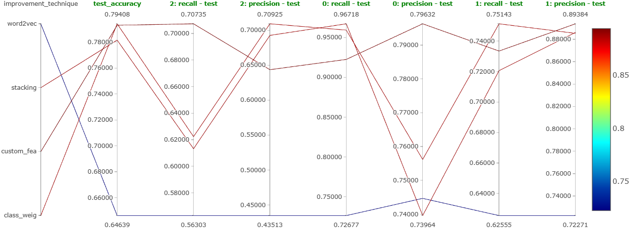
The decisive factor for class_weight was operational, not just metric-driven, it removes the undersampling step entirely. Less data thrown away means a more efficient training pipeline, and the model handles imbalance intrinsically.
Final model: LightGBM with class_weight="balanced", bag-of-words bigrams, max_features=1000, Optuna-tuned hyperparameters.
5 The DVC Pipeline
Everything in the training side of the system is wired into a DVC pipeline so dvc repro reproduces the whole thing end-to-end from raw data in S3 to a registered model in MLflow.
5.1 Pipeline Shape
%%{init: {'theme':'dark', 'themeVariables': { 'primaryColor': '#375a7f', 'primaryTextColor': '#fff', 'primaryBorderColor': '#6c757d', 'lineColor': '#adb5bd'}}}%%
flowchart TB
 S3[(S3: raw_data.csv)] --> DI[data_ingestion.py]
 DI --> RAW[data/raw/<br/>train.csv, test.csv]
 RAW --> DP[data_preprocessing.py]
 DP --> INT[data/interim/<br/>train.csv, test.csv]
 INT --> FE[feature_engineering.py]
 FE --> PROC[data/processed/<br/>X_train, X_test, y_train, y_test]
 FE --> VEC[models/vectorizer.pkl]
 PROC --> MT[model_training.py]
 MT --> MDL[models/model.pkl]
 PROC --> ME[model_evaluation.py]
 MDL --> ME
 VEC --> ME
 ME --> EXP[experiment_info.json]
 ME --> MLF1[(MLflow:<br/>metrics + artifacts)]
 EXP --> MR[model_registration.py]
 MR --> MLF2[(MLflow Registry:<br/>Staging)]

 style S3 fill:#375a7f,stroke:#fff,color:#fff
 style MLF1 fill:#00bc8c,stroke:#fff,color:#fff
 style MLF2 fill:#00bc8c,stroke:#fff,color:#fff
5.2 Stage-by-Stage
| Stage | Module | What it does |
|---|---|---|
| Ingestion | data_ingestion.py |
Pulls raw CSV from S3; drops NaNs, duplicates, and empty comments; does a stratified train/test split; writes data/raw/. |
| Preprocessing | data_preprocessing.py |
Lowercases, removes URLs, removes stop words (keeping not/but/however/no/yet), lemmatizes; writes data/interim/. |
| Feature engineering | feature_engineering.py |
Fits CountVectorizer(ngram_range=(1,2), max_features=1000) on train, transforms both splits, persists the vectorizer to models/vectorizer.pkl. |
| Training | model_training.py |
Fits LGBMClassifier with the tuned hyperparameters; persists models/model.pkl. |
| Evaluation | model_evaluation.py |
Scores on test; logs params, metrics, confusion matrix, model with signature, and vectorizer to MLflow; writes experiment_info.json with run ID and model path. |
| Registration | model_registration.py |
Reads experiment_info.json, registers the model, transitions to Staging. |
Two supporting files hold it all together: dvc.yaml defines stage dependencies and outputs, and params.yaml holds every tunable (train/test split ratio, CountVectorizer settings, LGBM hyperparameters) so they can be changed without touching code.
6 Backend: FastAPI
6.1 Responsibilities
The FastAPI app (backend/app.py) is deliberately thin. Its job is to:
- Load the Production model from MLflow and the vectorizer from disk once, at startup.
- Accept comments from the extension.
- Preprocess → vectorize → predict.
- Generate the three server-side visualizations (pie chart, word cloud, monthly trend).
- Return JSON or PNG responses.
6.2 Endpoint Surface
%%{init: {'theme':'dark', 'themeVariables': { 'primaryColor': '#375a7f', 'primaryTextColor': '#fff', 'primaryBorderColor': '#6c757d', 'lineColor': '#adb5bd'}}}%%
flowchart LR
 subgraph Core["Prediction endpoints"]
 P1[/POST /predict/]
 P2[/POST /predict_with_timestamps/]
 end
 subgraph Viz["Visualization endpoints"]
 V1[/POST /generate_chart/]
 V2[/POST /generate_wordcloud/]
 V3[/POST /generate_trend_graph/]
 end

 IN1[["comments: list[str]"]] --> P1
 IN2[["comments + timestamps"]] --> P2
 IN3[["sentiment counts"]] --> V1
 IN4[["comments"]] --> V2
 IN5[["timestamped labels"]] --> V3

 P1 --> OUT1[["[{comment, sentiment}]"]]
 P2 --> OUT2[["[{comment, sentiment, ts}]"]]
 V1 --> OUT3[["pie chart PNG"]]
 V2 --> OUT4[["word cloud PNG"]]
 V3 --> OUT5[["line chart PNG"]]
6.3 Preprocessing Mirror
A subtle but critical detail: the preprocessing applied to incoming comments must exactly match the training-time preprocessing. Any divergence (a different stop-word list, a missing lemmatization step) silently corrupts inference. The backend reuses the same logic (lowercase, newline/non-alphanumeric scrub, stop-word removal with the five exceptions, WordNet lemmatization) that the DVC data_preprocessing.py stage uses.
6.4 Startup-Time Resource Loading
# Conceptual, see backend/app.py for the real thing
@app.on_event("startup")
def load_resources():
    global model, vectorizer
    mlflow.set_tracking_uri(DAGSHUB_URI)
    model = mlflow.pyfunc.load_model("models:/youtube_comments_analyzer/Production")
    vectorizer = joblib.load("/app/models/vectorizer.pkl")
This has two consequences. First, each container is stateful in the sense that its model reference is pinned at startup. A freshly promoted model in the registry will not be picked up until the containers are restarted, which CodeDeploy handles during its rolling deploy. Second, startup latency includes model download time, which is why the ALB’s health-check grace period matters.
6.5 Error Handling
The endpoints catch and report: malformed JSON input, preprocessing failures (e.g., non-string entries in the comments array), vectorizer-shape mismatches, and model prediction errors. Each produces a structured HTTP error response rather than a 500 with a stack trace.
6.6 Example Request/Response
// POST /predict
{
    "comments": [
        "I love this video",
        "This was terrible and boring"
    ]
}
// Response
[
{"comment": "I love this video", "sentiment": 1},
{"comment": "This was terrible and boring","sentiment": -1}
]7 Frontend: The Chrome Extension
7.1 Anatomy of the Extension
A Chrome extension at its minimum is three files:
| File | Role |
|---|---|
manifest.json |
Declares the extension’s permissions, icons, popup page, and (importantly) the domains it may talk to (the ALB’s DNS name, YouTube’s API, and any image sources). |
popup.html |
The UI shown when the user clicks the toolbar icon. Hosts containers for the sentiment boxes, the three images, the metrics, and the top-25 comment list. Styled with inline CSS in a dark theme. |
popup.js |
All the logic: URL validation, calls to the YouTube Data API, calls to the FastAPI backend, DOM rendering. |
A fourth file, secrets.json, holds the YouTube Data API key. It is .gitignore’d.
7.2 Client-Side Flow
%%{init: {'theme':'dark', 'themeVariables': { 'primaryColor': '#375a7f', 'primaryTextColor': '#fff', 'primaryBorderColor': '#6c757d', 'lineColor': '#adb5bd'}}}%%
flowchart TB
 START([Popup opens]) --> CHK{URL is<br/>YouTube video?}
 CHK -- No --> MSG1[Show 'not a YouTube video']
 CHK -- Yes --> VID[Extract videoId]
 VID --> FC[fetchComments<br/>up to 500]
 FC --> GSP[getSentimentPredictions<br/>POST /predict_with_timestamps]
 GSP --> SPLIT{Distribute to UI renderers}

 SPLIT --> PCT[Compute sentiment %]
 SPLIT --> CHART[fetchAndDisplayChart<br/>→ /generate_chart]
 SPLIT --> WC[fetchAndDisplayWordCloud<br/>→ /generate_wordcloud]
 SPLIT --> TR[fetchAndDisplayTrendGraph<br/>→ /generate_trend_graph]
 SPLIT --> MET[Compute metrics<br/>total, unique authors,<br/>avg words, avg sentiment score]
 SPLIT --> TOP[Render top-25 comments]

 PCT --> DONE([Render dashboard])
 CHART --> DONE
 WC --> DONE
 TR --> DONE
 MET --> DONE
 TOP --> DONE
7.3 The “Average Sentiment Score” Metric
Among the four headline metrics, the only non-trivial one is the average sentiment score, mapped onto a 0-10 scale where higher is more positive:
\[ \text{avg score} \;=\; \frac{(+1)\,c_{+} + 0 \cdot c_{0} + (-1)\,c_{-}}{c_{+} + c_{0} + c_{-}} \times 10 \]
The other three (total comments, unique commenters, average words per comment) are computed directly from the YouTube API response without hitting the backend.
7.4 Iterative Build
The extension was built as a sequence of seven progressively-richer prototypes, each a separate commit:
- Hard-coded two-comment prototype, verifying the extension can POST to the backend.
- URL checker / videoId extraction.
- YouTube Data API wired up for comment counts.
- Sentiment percentages on 100 comments.
- 500-comment fetch, top-25 display, dark-theme styling.
- Pie chart from
/generate_chart. - Word cloud, monthly trend, headline metrics, the current production surface.
8 CI/CD Pipeline
8.1 The Workflow at a Glance
%%{init: {'theme':'dark', 'themeVariables': { 'primaryColor': '#375a7f', 'primaryTextColor': '#fff', 'primaryBorderColor': '#6c757d', 'lineColor': '#adb5bd'}}}%%
flowchart TB
 TRIG[on: push] --> CK[Checkout]
 CK --> PY[Setup Python 3.11]
 PY --> CACHE[Cache pip]
 CACHE --> DEPS[Install deps + dvc-s3]
 DEPS --> REPRO[dvc repro]
 REPRO --> DPUSH[dvc push → S3]
 DPUSH --> GIT[git add/commit/push<br/>as github-actions bot]
 GIT --> T_LOAD[Test: model loading]
 T_LOAD --> T_SIG[Test: model signature]
 T_SIG --> T_PERF[Test: performance ≥ 0.75]
 T_PERF --> PROMO[Promote Staging → Production]
 PROMO --> FASTAPI[Start FastAPI + wait]
 FASTAPI --> T_API[Test: FastAPI endpoints]
 T_API --> ECR_LOGIN[Log in to ECR]
 ECR_LOGIN --> D_BUILD[docker build]
 D_BUILD --> D_TAG[docker tag]
 D_TAG --> D_PUSH[docker push → ECR]
 D_PUSH --> ZIP[Zip deploy bundle]
 ZIP --> S3UP[Upload to S3]
 S3UP --> DEPLOY[aws deploy create-deployment]

 style PROMO fill:#00bc8c,stroke:#fff,color:#fff
 style DEPLOY fill:#00bc8c,stroke:#fff,color:#fff
 style T_PERF fill:#e74c3c,stroke:#fff,color:#fff
8.2 Pipeline Reproduction
Running the DVC pipeline inside CI requires a handful of secrets and a little care to avoid runaway loops. The core step:
- name: Run DVC Pipeline
    env:
        AWS_ACCESS_KEY_ID: ${{ secrets.AWS_ACCESS_KEY_ID }}
        AWS_SECRET_ACCESS_KEY: ${{ secrets.AWS_SECRET_ACCESS_KEY }}
        AWS_DEFAULT_REGION: us-east-2
        RAW_DATA_S3_BUCKET_NAME: ${{ secrets.RAW_DATA_S3_BUCKET_NAME }}
        RAW_DATA_S3_KEY: ${{ secrets.RAW_DATA_S3_KEY }}
        DAGSHUB_USER_TOKEN: ${{ secrets.DAGSHUB_USER_TOKEN }}
    run: dvc repro
After dvc repro, artifacts are pushed to the S3 DVC remote:
- name: Push DVC-tracked Data to Remote
    run: dvc push
The pipeline also modifies dvc.lock and possibly other tracked files. Those changes need to land back on the repo. The workflow configures a bot identity and commits, but only if the actor wasn’t itself the bot, which is the standard trick to avoid an infinite CI loop:
- name: Commit Changes
    if: ${{ github.actor != 'github-actions[bot]' }}
    run: git commit -m "Automated commit of DVC outputs" || echo "No changes"
8.3 Model Tests
Three staged tests, each gating the next:
- Model loading via
tests/test_model_loading.py. Fetches the just-registered Staging model from MLflow and asserts it’s usable. - Model signature via
tests/test_model_signature.py. A mismatch between expected input shape/dtype and the model’s signature is one of the sneakiest ways to break production. This test pushes a preprocessed sample through and verifies both input and output shapes. - Performance via
tests/test_model_performance.py. Scores the model on a validation slice and fails if accuracy, precision, recall, or F1 falls below 0.75.
Pass all three → scripts/promote_model.py transitions the Staging model to Production and archives any currently-Production model.
8.4 API Tests
Once the model is in Production, the workflow spins up FastAPI in the background and waits for the port to become available:
- name: Wait for FastAPI to be Ready
    run: |
        for i in {1..10}; do
            nc -z localhost 5000 && echo "FastAPI is up!" && exit 0
            echo "Waiting for FastAPI..." && sleep 3
        done
    echo "FastAPI server failed to start" && exit 1
Then tests/test_fast_api.py hits each of the five endpoints with dummy payloads and asserts on status codes and response shapes.
9 Containerization
9.1 Dockerfile
The image starts from python:3.11-slim to keep size down:
FROM python:3.11-slim

WORKDIR /app/backend

# OpenMP, needed by LightGBM
RUN apt-get update && apt-get install -y libgomp1

# Copy only what's needed for inference
COPY backend/ /app/backend/
COPY models/ /app/models/

# Inference-specific requirements (kept separate from training reqs)
RUN pip install -r requirements.txt

# NLTK assets needed for preprocessing at inference time
RUN python -m nltk.downloader stopwords wordnet

EXPOSE 5000
CMD ["uvicorn", "app:app", "--host", "0.0.0.0", "--port", "5000"]
Two things worth calling out:
backend/requirements.txtis intentionally a trimmed version of the project’srequirements.txt: only the libraries the inference server actually imports. Training-only libraries (Optuna, DVC, MLflow extras beyond the model-loading client, matplotlib-for-EDA, spaCy, etc.) are omitted. This keeps the final image size reasonable.libgomp1is easy to forget. LightGBM binaries that were linked against OpenMP will fail at import time on slim base images without it.
9.2 Local Build and Sanity Test
docker build -t sushrutgaikwad/youtube-comments-analyzer .
docker run -p 8888:5000 \
    -e AWS_ACCESS_KEY_ID=DUMMY \
    -e AWS_SECRET_ACCESS_KEY=DUMMY \
    -e DAGSHUB_USER_TOKEN=DUMMY \
    sushrutgaikwad/youtube-comments-analyzer
Port 5000 inside the container is exposed on 8888 on the host. The dummy env vars are enough to let the container start; real AWS/DagsHub credentials are only needed if you actually want it to load the Production model from the registry.
9.3 Pushing to ECR
After an aws configure, the standard four ECR commands (all automated in the workflow):
aws ecr get-login-password --region us-east-2 \
    | docker login --username AWS \
    --password-stdin 872515288060.dkr.ecr.us-east-2.amazonaws.com
docker build -t youtube-comments-analyzer .
docker tag youtube-comments-analyzer:latest \
    872515288060.dkr.ecr.us-east-2.amazonaws.com/youtube-comments-analyzer:latest
docker push 872515288060.dkr.ecr.us-east-2.amazonaws.com/youtube-comments-analyzer:latest
In CI these become four GitHub Actions steps, each gated on if: success() so a failure earlier in the workflow (say, a model test failing) aborts the build before it can ship a broken image.
10 Deployment: AWS EC2 + CodeDeploy
10.1 Deployment Topology
%%{init: {'theme':'dark', 'themeVariables': { 'primaryColor': '#375a7f', 'primaryTextColor': '#fff', 'primaryBorderColor': '#6c757d', 'lineColor': '#adb5bd'}}}%%
flowchart TB
 USER[User] -- HTTPS --> DNS[Route 53 / ALB DNS]
 DNS --> ALB[Application Load Balancer<br/>health checks]

 subgraph ASG["Auto Scaling Group (2-3 instances)"]
 direction LR
 I1[EC2 instance 1<br/>CodeDeploy agent<br/>Docker: FastAPI:5000]
 I2[EC2 instance 2<br/>CodeDeploy agent<br/>Docker: FastAPI:5000]
 I3[EC2 instance 3<br/>on scale-out]
 end

 ALB --> I1
 ALB --> I2
 ALB -. scale-out .-> I3

 subgraph CD_STACK["Deployment control plane"]
 CDAPP[CodeDeploy application]
 CDGRP[Deployment group<br/>OneAtATime]
 S3B[(S3:<br/>deployment.zip)]
 ECR[(ECR:<br/>latest image)]
 end

 CDGRP --> ASG
 S3B --> CDGRP
 I1 -.->|docker pull| ECR
 I2 -.->|docker pull| ECR
 I3 -.->|docker pull| ECR
10.2 The Two IAM Roles
Deployment hinges on two separate IAM roles:
- EC2 instance role, attached to the launch template. Lets each instance pull images from ECR and be managed by CodeDeploy. Policies:
AmazonEC2ContainerRegistryReadOnlyAmazonEC2RoleforAWSCodeDeploy
- CodeDeploy service role, lets CodeDeploy itself manipulate the Auto Scaling Group, target groups, and load balancer. Policy:
AWSCodeDeployRole.
10.3 Launch Template + User Data
The launch template bakes the CodeDeploy agent into every instance via its user-data script:
#!/bin/bash
sudo apt-get update -y
sudo apt-get install ruby -y
wget https://aws-codedeploy-us-east-2.s3.us-east-2.amazonaws.com/latest/install
chmod +x ./install
sudo ./install auto
sudo service codedeploy-agent start
After the ASG launches, sudo service codedeploy-agent status on each instance confirms the agent is running.
10.4 Auto Scaling Group Configuration
- Size: min 2, desired 2, max 3.
- Distribution: Balanced best-effort across AZs.
- Load balancer: new internet-facing Application Load Balancer, new target group, ELB health checks enabled.
- Scaling policy: target tracking on average CPU utilization, target value 50%, instance warm-up 300s.
10.5 CodeDeploy Application & Deployment Group
- Compute platform: EC2/On-premises.
- Deployment type: In-place.
- Environment: pointed at the ASG above.
- Deployment configuration:
CodeDeployDefault.OneAtATime, one instance taken out of rotation at a time, preventing the fleet from ever being fully down. - Load balancer: the ALB + target group from the ASG.
10.6 The Deployment Bundle
Three files make up the deployment bundle that CodeDeploy consumes:
10.6.1 appspec.yml
version: 0.0
os: linux
files:
    - source: /
      destination: /home/ubuntu/app
hooks:
    BeforeInstall:
        - location: deploy/scripts/install_dependencies.sh
          timeout: 300
          runas: ubuntu
    ApplicationStart:
        - location: deploy/scripts/start_docker.sh
          timeout: 300
          runas: ubuntu
10.6.2 deploy/scripts/install_dependencies.sh
Idempotent setup of the instance: Docker, AWS CLI, user permissions.
#!/bin/bash
export DEBIAN_FRONTEND=noninteractive
sudo apt-get update -y
sudo apt-get install -y docker.io
sudo systemctl start docker && sudo systemctl enable docker
sudo apt-get install -y unzip curl

curl "https://awscli.amazonaws.com/awscli-exe-linux-x86_64.zip" -o "/home/ubuntu/awscliv2.zip"
unzip -o /home/ubuntu/awscliv2.zip -d /home/ubuntu/
sudo /home/ubuntu/aws/install

sudo usermod -aG docker ubuntu
rm -rf /home/ubuntu/awscliv2.zip /home/ubuntu/aws
10.6.3 deploy/scripts/start_docker.sh
Pull the latest image, cleanly replace any running container, bind host port 80 to container port 5000 so the ALB’s HTTP listener lines up with the app:
#!/bin/bash
exec > /home/ubuntu/start_docker.log 2>&1

echo "Logging in to ECR..."
aws ecr get-login-password --region us-east-2 \
    | docker login --username AWS \
    --password-stdin 872515288060.dkr.ecr.us-east-2.amazonaws.com

echo "Pulling Docker image..."
docker pull 872515288060.dkr.ecr.us-east-2.amazonaws.com/youtube-comments-analyzer:latest

echo "Checking for existing container..."
if [ "$(docker ps -q -f name=youtube-comments-analyzer)" ]; then
    docker stop youtube-comments-analyzer
fi
if [ "$(docker ps -aq -f name=youtube-comments-analyzer)" ]; then
    docker rm youtube-comments-analyzer
fi

echo "Starting new container..."
docker run -d -p 80:5000 --name youtube-comments-analyzer \
    872515288060.dkr.ecr.us-east-2.amazonaws.com/youtube-comments-analyzer:latest

echo "Container started successfully."
10.7 Wiring It All to CI
The final three steps of ci-cd.yaml zip the bundle, upload to S3, and trigger CodeDeploy:
- name: Zip Files for Deployment
    if: success()
    run: zip -r deployment.zip appspec.yml deploy/scripts/install_dependencies.sh deploy/scripts/start_docker.sh

- name: Upload Zip File to S3
    if: success()
    run: aws s3 cp deployment.zip s3://yt-comments-analyzer-codedeploy-bucket/deployment.zip

- name: Deploy to AWS CodeDeploy
    if: success()
    run: |
        aws deploy create-deployment \
        --application-name youtube-comments-analyzer \
        --deployment-config-name CodeDeployDefault.OneAtATime \
        --deployment-group-name youtube-comments-analyzer-deployment-group \
        --s3-location bucket=yt-comments-analyzer-codedeploy-bucket,key=deployment.zip,bundleType=zip \
        --file-exists-behavior OVERWRITE \
        --region us-east-2
11 Observability (Planned)
The current deployment is covered by AWS CloudWatch for infrastructure-level telemetry: instance CPU, ALB request counts, target group health, container logs via the Docker driver. That’s enough to know whether the fleet is alive; it is not enough to know whether the model is alive and behaving.
The intended next step is a model-observability layer. The sketch:
%%{init: {'theme':'dark', 'themeVariables': { 'primaryColor': '#375a7f', 'primaryTextColor': '#fff', 'primaryBorderColor': '#6c757d', 'lineColor': '#adb5bd'}}}%%
flowchart LR
 API[FastAPI<br/>/metrics endpoint] -->|scrape| PROM[Prometheus]
 API --> CW[CloudWatch Logs]
 PROM --> GRAF[Grafana dashboards]
 CW --> GRAF

 subgraph Metrics["Planned metrics"]
 M1[Inference latency<br/>p50/p95/p99]
 M2[Request throughput]
 M3[Predicted class<br/>distribution]
 M4[Input length<br/>distribution]
 M5[Error rate per<br/>endpoint]
 end

 API -.emits.-> M1 & M2 & M3 & M4 & M5

 style PROM fill:#555,stroke:#fff,color:#fff,stroke-dasharray: 5 5
 style GRAF fill:#555,stroke:#fff,color:#fff,stroke-dasharray: 5 5
Dashed components are planned, not shipped. The Grafana dashboards would compare live predicted-class distribution and input-length distribution against their training-time counterparts to catch data drift early. Examples include a shift toward shorter comments, or a sudden collapse of the negative-class prediction rate the way the baseline model did.
12 What’s Deliberately Out of Scope (For Now)
A few things that are mentioned elsewhere as “we could do this” but were intentionally not pursued in v1:
- Multilingual support. Detecting and handling non-English and code-switched comments would require a very different feature pipeline (likely multilingual embeddings) and a much larger labelled corpus. Punted.
- Sarcasm detection. Genuinely open research. A bag-of-words LightGBM is not going to solve this.
- A deep-learning model (transformer fine-tune). Experiment 5 showed all classical ML families topping out in a similar range, a transformer would plausibly improve absolute accuracy, but at a latency cost that would require either async inference or a bigger instance class, and the current accuracy/latency trade-off is acceptable for the product goal.
- Stacking ensemble in production. Experiment 6 showed it was competitive on accuracy but the four-base-model latency was unacceptable.
13 Repository Map
| Repo | Role |
|---|---|
youtube-comments-analyzer |
Training pipeline (DVC), FastAPI backend, Dockerfile, CI/CD workflow, deploy scripts. |
youtube-comments-analyzer-frontend |
Chrome extension (manifest.json, popup.html, popup.js). |
Key directories in the backend repo:
youtube-comments-analyzer/
├── youtube_comments_analyzer/    # Python package: DVC pipeline stages
│   ├── data_ingestion.py
│   ├── data_preprocessing.py
│   ├── feature_engineering.py
│   ├── model_training.py
│   ├── model_evaluation.py
│   └── model_registration.py
├── backend/                      # FastAPI app + inference-only requirements
│   ├── app.py
│   └── requirements.txt
├── tests/                        # pytest: model loading, signature, perf, API
├── scripts/                      # deployment scripts
│   └── promote_model.py
├── notebooks/                    # 01-21: EDA through final model selection
├── deploy/scripts/               # install_dependencies.sh, start_docker.sh
├── .github/workflows/            # CI/CD workflow
│   └── ci-cd.yaml
├── dvc.yaml                      # DVC pipeline definition
├── params.yaml                   # Hyperparameters and model configs
├── appspec.yml                   # CodeDeploy application specification
├── Dockerfile                    # Docker image definition
└── requirements.txt              # Production dependencies
14 Closing Thoughts
Two things stand out in retrospect.
The classical ML ceiling is real but liveable. Four very different model families (trees, linear, kernel) converged to the same accuracy band. That’s a signal that the data preprocessing and feature representation are the binding constraint, not the model family. That is exactly the kind of finding that would justify a feature-engineering investment (or a switch to learned embeddings) rather than another round of HPT. The decision to ship LightGBM with class_weight="balanced" was as much about operational simplicity as about metric wins.
The MLOps plumbing is where the project’s real leverage is. The model accuracy isn’t state-of-the-art. But the retrain-test-promote-deploy loop means a better model (whether it comes from new data, a transformer replacement, or a completely different approach) can be dropped in without rewriting anything downstream. That’s the piece that generalizes beyond this one project.