Spotify Hybrid Song Recommender
A Spotify recommender system built using a hybrid approach of content based filtering and collaborative filtering.
Introduction
What are Recommender Systems?
Recommender systems are algorithms that recommend content (e.g., books, movies, TV shows, etc.) to a user based on their preference and current behavior. Colloquially, a recommender system is like a user’s friend who knows their taste, current behavior, and currently what is going on in their life. Based on this knowledge, this friend can recommend content to the user that the user can potentially find interesting. Note that the taste of the user is dynamic (i.e., it keeps changing). The friend takes into consideration user’s current taste to give the best recommendations. The same is true with recommender systems.
Recommender systems are used in a variety of industries. Some of them are:
- Media Streaming: Netflix, Amazon Prime, YouTube, Spotify, etc.
- E-Commerce: Amazon, Flipkart, etc.
- Social Media: Facebook, Instagram, etc.
Why Recommender Systems?
Let us take the example of movie streaming. Why not simply sort all the movies lexicographically and give it to the user? For instance, we can create web pages for all movies starting with the letter “A”, next web page for all the movies starting with the letter “B”, and so on. There are multiple problems with this approach. Some of the main ones are the following.
The Need of User to be Extremely Specific
The user will have to know the exact movie they want to watch so that they can search for it and watch it. This is like the proverbial needle in a haystack problem.
No Way to Search for Similar Content
Once the user watches the specific movie they want to watch, there is no way for them to search for a unknown movie which is similar to the movie they just watched. As these movies are similar, the user will potentially like it. This will increase the user’s engagement with the streaming platform.
This is why recommender systems play a crucial role in today’s industry.
Types of Recommender Systems
We will discuss about recommender systems starting from the very basic to the relatively modern.
Popularity-Based Recommender System
As the name suggests, this recommender system simply recommends the user the content that is the “most popular”, e.g., highly rated, watched by most, currently trending, etc. It is so simple that we do not need any machine learning algorithm here. In the movie streaming platform context, we simply need a database that contains the movies along with their user ratings. So, providing recommendation in this system simply amounts to grouping by these ratings, sorting by the average rating in descending order, and displaying the top-\(k\) (e.g., top-10) movies to the user. Further, instead of user ratings, we can also group by the revenue earned by the movie, or some other column. A simple filter, e.g., based on language, can also be applied by asking the user their preferred language.
Advantages
The advantages of this recommender system are the following:
- Easy to implement: As discussed, this system simply amounts to grouping by a particular column (e.g., user ratings, revenue earned, etc.) and display some top-\(k\) movies in descending order of that column.
- Easy to tackle cold-start problem: The cold start problem in the movie streaming context is recommending movies to a new user. As this user is new, their taste, e.g., their past viewing history, is unknown. So recommending movies that this user likes is difficult. However if we are simply displaying the top-10 movies to all users, then this problem is easily solved.
- Highly scalable: No matter how much the movie catalogue or the user population increases, the logic still remains easy to implement.
Disadvantages
There are some serious disadvantages of this recommender system. Some of them are the following:
- No personalized recommendations: This system does not address the diversity in user taste. Just because most users have rated a movie highly doesn’t mean that all users will like it.
- Bias: If there is a genuinely good movie on the streaming platform but it is seen by very few people, and rated by even fewer, then this movie will rank a lot lower on the scale as compared to a movie which is not that good but is seen by many and also rated by many due to starring a popular actor. So, such a system is biased against some niche but really good movies.
- Lack of Diversity: If a multilingual user selects that they prefer watching movies in English, then the system won’t be able to recommend the user good movies in other languages.
Content-Based Recommender System
A content-based recommender system recommends content to a user that is similar to the content that is already consumed by them.
Advantages
- Recommends similar content: As mentioned before, this system recommends content that is similar (with respect to the metadata) to the content already consumed by the user. This adds a personalized touch to the recommendation which increases user engagement.
- Recommendations solely dependent on user habits: For example, if a user watches a lot of data science related videos on YouTube, then they will be recommended more of such videos. If in future they start watching web development related videos, then the recommendations will now shift to web development related videos. So, the user habits determine the recommendations.
Disadvantages
- Overspecialized recommendations: Say a user studies the entire day by watching data science related videos on YouTube. However, when they unwind in the evening, they may want some entertainment (e.g., comedy). However, they won’t be shown such content unless they search for it. The system cannot recommend content other than the content that the user is currently watching or have watched before. So, the recommendations the user gets are too specialized.
- No diversity: This is connected to the previous point. Overspecialization will lead to less diverse recommendations.
- Cold start problem: Whenever a new user joins the platform, the system won’t know what to recommend as it does not know about the user’s history and search habits.
Working of Content-Based Recommender System
Consider the example of movie streaming platform. Each row in the data has features of a particular movie. Say there are two features, namely ratings and duration. Consider the toy dataset shown in Table 1.
| Movie name | Rating | Duration (hrs.) |
|---|---|---|
| Movie A | 4 | 2 |
| Movie B | 5 | 1.5 |
| Movie C | 2 | 3.5 |
Table 1: Ratings and durations of movies.
This can be viewed as vectors on a coordinate plane, as shown in Figure 1.

Just by looking at the figure, it is clear that Movie A and Movie B are closer to each other, and hence are more “similar” to each other. So if a user watches Movie A, we can recommend them Movie B. We will discuss how this “similarity” is calculated later.
Collaborative Filtering
A collaborative filtering recommender system is based on user-item interation. To put it more simply, this recommender system is based on the usage and taste of other users that are similar to the users to whom we want to give recommendations. Collaborative filtering can be further divided into two types.
User-Based Collaborative Filtering
Consider the following movie streaming scenario. Say we have 5 users, \(U_1\), \(U_2\), …, \(U_5\), and 3 movies, \(M_1\), \(M_2\), and \(M_3\). The ratings given by each user to each of the movies is indicated in Table 2.
| $$M_1$$ | $$M_2$$ | $$M_3$$ | |
|---|---|---|---|
| $$U_1$$ | 3 | 4 | – |
| $$U_2$$ | – | 4 | – |
| $$U_3$$ | 2 | 5 | 4 |
| $$U_4$$ | – | – | – |
| $$U_5$$ | 3 | 3.5 | 2 |
Table 2: User–movie rating matrix.
Note that the “–” in the table indicates that the corresponding user didn’t rate that particular movie. Now, say the platform wants to recommend movies to user \(U_2\) who has just watched a single movie, i.e., \(M_2\). To do this we follow the following steps:
- We will calculate the similarity of this user \(U_2\) with all the other users.
- Select the user that is the most similar to \(U_2\).
- Say \(U_1\) is the user that is the most similar to \(U_2\). We will recommend \(U_2\) the movie that is not watched by them but is watched by \(U_1\) and is also highly rated by \(U_1\).
This movie is \(M_1\). Hence, we will recommend the movie \(M_1\) to the user \(U_2\).
User-based collaborative filtering is used when the number of items is far greater than the number of users. Remember that in this type of collaborative filtering, each row in the matrix stands for a particular user.
Item-Based Collaborative Filtering
This is very similar to user-based collaborative filtering. The only difference is that there we found similarity between users, whereas here we find similarity between items. Say we have 4 items, \(I_1\), \(I_2\), …, \(I_4\), and 3 users \(U_1\), \(U_2\), and \(U_3\). Consider the matrix shown in Table 3. This table indicates whether a particular item is liked by a user (using Boolean values).
| $$U_1$$ | $$U_2$$ | $$U_3$$ | |
|---|---|---|---|
| $$I_1$$ | 1 | 1 | 1 |
| $$I_2$$ | 1 | 1 | 0 |
| $$I_3$$ | 0 | 0 | 0 |
| $$I_4$$ | 0 | 0 | 1 |
Table 3: Binary user-item preference matrix.
Now we calculate similarity between items. We can see that item \(I_1\) is liked by users \(U_1\), \(U_2\), and \(U_3\); item \(I_2\) is liked by users \(U_1\) and \(U_2\); and item \(I_4\) is liked by user \(U_3\). We can see that items liked by user \(U_2\) are also liked by user \(U_1\). So, if right now someone is consuming item \(I_2\), then they will be recommended item \(I_1\) as it is similar to \(I_2\). As we can see, the recommendations here are based on the similarity of items.
Item-based collaborative filtering is used when the number of users is far greater than the number of items. Remember that in this type of collaborative filtering, each row in the matrix stands for a particular item.
Advantages
- Diversity: This recommender system can expose a user to content they aren’t exposed to yet, i.e., new content.
- Better recommends as the data size increases: In the context of a movie streaming platform, as the number of movies and number of users increase, the interaction between them will become richer, improving the recommendation system for all users.
- Non-reliance on metadata: This system does not rely on the metadata.
Disadvantages
- Cold start problem: For a new user would have watched very few, if any, movies. Similarly, very few users, if any, would have rated or watched a new movie. So, there won’t be a lot of information on these new users and new movies. Hence, the recommendation system will have a hard time in giving recommendations.
- Computationally expensive: The number of steps carried out in giving recommendations using collaborative filtering is significantly more than other recommendation systems. Hence, it is computationally expensive.
- Large datasets: The item-user interaction matrix can be massive.
Hybrid Recommendation System
A hybrid recommendation system combines multiple types of recommender systems into a single recommender system. In doing this, it eliminates the disadvantages of all of these recommendation systems and retains their advantages. By looking at the advantages of all the recommender systems we have discussed so far, it is clear that this will happen since for each recommender system there is another recommender system whose advantages address its disadvantages. We will work on a hybrid recommender system that combines content-based filtering with collaborative filtering.
Working of Hybrid Recommender System
There are multiple approaches used to build a hybrid recommender system. We will be using a weighted approach. Let \(w_{\text{cb}}\) denote the weight of content-based filtering and \(w_{\text{cf}}\) denote the weight of collaborative filtering. We will choose these weights such that
\[\begin{equation*} w_{\text{cb}} + w_{\text{cf}} = 1 \end{equation*}\]These weights will be applied to the similarity scores.
Similarity Score
Similarity score can be calculated using various approaches. Distance-based similarity is very common. For instance, each movie will be a vector, and the distance (Euclidean, Manhattan, or cosine) between two movie vectors can be calculated. The lower this distance, the higher the similarity.
Another approach is using cosine similarity. We will be using this approach because of its two key advantages:
- It is immune to curse of dimensionality, i.e., no matter how high dimensional (i.e., a lot of features) the data is, this can be calculated easily.
- It is bounded between \(-1\) to \(1\).
- \(-1\) means highest dissimilarity,
- \(0\) means no similarity,
- \(1\) means highest similarity.
The cosine similarity between two vectors \(\mathbf{v}_1\) and \(\mathbf{v}_2\) is given by
\[\begin{equation}\label{eq:cosine_similarity} \cos\left(\theta\right) = \frac{\mathbf{v}_1^{\intercal} \mathbf{v}_2}{\left\lvert\left\lvert \mathbf{v}_1 \right\rvert\right\rvert \left\lvert\left\lvert \mathbf{v}_2 \right\rvert\right\rvert} \end{equation}\]Recall that the numerator, i.e., \(\mathbf{v}_1^{\intercal} \mathbf{v}_2\), is nothing but the dot product between the vectors \(\mathbf{v}_1\) and \(\mathbf{v}_2\). So highest dissimilarity means that the vectors are at \(180^{\circ}\) (or opposite) to each other, no similarity means that the vectors are at \(90^{\circ}\) (or perpendicular) to each other, and highest similarity means the vectors are at \(0^{\circ}\) (or parallel) to each other.
Spotify Recommender System
We are replicating a scenario in which Spotify, which is a music streaming platform, is facing high customer churn rate. Spotify till now offers only popularity-based recommendations, i.e., music with the most play count. Due to the high churn rate, the platform is facing poor user engagement and poor user retention. They are switching to platforms that offer more personalized as well as a variety of recommendations. After quite a bit of brainstorming, it was decided that the currently used popularity-based recommender system will be replaced with a new hybrid recommender system such that the users get more personalized and a variety of recommendations. This should in turn help with the high customer churn rate as it will improve user engagement and retention.
From the Spotify database, we will use the following two datasets:
- Songs dataset: This has information about all the songs on Spotify, e.g., attributes, metadata, etc.
- User-Song Interaction dataset: This has information about how many times a particular user has played a particular song. This information is available for all users.
We will use the first dataset to build a content-based recommender system and the second to build a collaborative-filtering recommender system. Finally, we will combine both these systems to build a hybrid recommender system.
Goal of the Project
As mentioned before, the goal of the project is to improve user engagement and user retention on Spotify by providing personalized and a variety of recommendations. We will be achieving this goal by building a hybrid recommender system.
Data
The data is available on Kaggle, which can be checked out here. The songs dataset that was mentioned is named as the “Music Info”, which contains 50,683 songs (or tracks). The description of this data is shown in Table 4.
| Column | Description |
|---|---|
track_id | Unique identifier for each track (e.g., TRIOREW128F424EAF0). |
name | Title of the song or track. |
artist | Name of the primary performing artist or group. Unique artists: ≈ 8 300 |
spotify_preview_url | Direct link to Spotify’s 30-second audio preview for the track. |
spotify_id | Spotify’s unique identifier for the track (spotify:track: URI suffix). |
tags | Variable-length, comma-separated listener tags describing genre, mood, era, etc. Most frequent tags (top 10): rock, indie, electronic, alternative, pop, female_vocalists, alternative_rock, indie_rock, metal, classic_rock |
genre | Broad genre label inferred from metadata (may be blank if unknown). Categories (15): Blues, Country, Electronic, Folk, Jazz, Latin, Metal, New Age, Pop, Punk, Rap, Reggae, RnB, Rock, World |
year | Calendar year the track was first released (range 1900 – 2022). |
duration_ms | Total length of the track in milliseconds. |
danceability | Spotify audio feature measuring how suitable the track is for dancing (0.0 – 1.0; higher = more danceable). |
energy | Overall intensity and activity level of the track (0.0 – 1.0; higher = more energetic). |
key | Estimated musical key using Pitch-Class notation (0 = C, 1 = C♯/D♭, …, 11 = B). Categories (12): 0, 1, 2, 3, 4, 5, 6, 7, 8, 9, 10, 11 |
loudness | Average loudness of the track in decibels relative to full scale (dBFS; typically negative). |
mode | Musical modality of the track. Categories: 1 = Major (≈ 63%), 0 = Minor (≈ 37%) |
speechiness | Proportion of spoken words in the track (0.0 – 1.0; higher values = more speech-like content). |
acousticness | Likelihood that the track is acoustic (0.0 – 1.0; higher = more acoustic). |
instrumentalness | Probability that the track contains no vocals (0.0 – 1.0; values > 0.5 suggest instrumental). |
liveness | Probability the track was performed live (0.0 – 1.0; higher = greater live-audience presence). |
valence | Musical positiveness conveyed by the track (0.0 = sad/angry, 1.0 = happy/cheerful). |
tempo | Estimated overall tempo of the track in beats per minute (BPM). |
time_signature | Estimated time-signature expressed as beats per bar. Categories: 4 (≈ 89%), 3, 5, 1, 0 |
Table 4: Column-wise description of the "Music Info" dataset.
Using this data, we will build the content-based filtering recommender system.
The user-song interaction dataset is named “User Listening History”, which has 9,711,301 records. The description of this data is shown in Table 5.
| Column | Description |
|---|---|
track_id | Unique identifier for each track (e.g., TRIRLYL128F42539D1). |
user_id | SHA-1–like hexadecimal hash uniquely identifying a user (e.g., b80344d063b5ccb3212f76538f3d9e43d87dca9e). |
playcount | Integer representing how many times the given user has listened to the track. |
Table 5: Column-wise description of the "User Listening History" dataset.
Using this, we will build the collaborative filtering recommender system. Further, we can also see that the songs dataset and the user-song interaction dataset has the column track_id in common. So they can be joined on this column.
Improving Business Metrics
Spotify broadly has two sources of revenue as it has two types of users:
- Revenue from free users: Free users on Spotify are shown advertisements.
- Revenue from subscribed users: Subscribed users pay fees to Spotify to make their experience advertisement free.
User Engagement
Once the users are provided with personalized and a variety of recommendations, user engagement with the platform will improve. This will, by definition, make the user listen to more songs. Free users will be shown an advertisement after they listen to a certain number of songs, which will generate revenue. If the user wants an advertisement free experience, they can subscribe. So, as the number of free users increase, the number of subscribed users will also increase. This will again generate revenue.
Click-Through Rate (CTR)
This is closely tied with user engagement. If CTR increases, so will user engagement. If a user, while listening, is shown 10 recommendations, and they choose the next song based on these recommendations, then it is considered as 1 click. And we want the user to select the next song from these recommendations. When the user is presented with more personalized and a variety of recommendations, they will like it more, and the probability that they will pick one of the songs from the recommendations as their next song also increases.
User Conversion
This is, again, linked to user engagement. If a free user is a regular user, they will be shown more advertisements. So, it is likely that they will buy a subscription plan. This is how free users can be converted to subscribed users. This will increase the users with subscription.
Lower Churn Rate
If a user is provided with good recommendations, then they will choose to stick with the platform and renew the subscription. So, a good recommender system will also lower the churn rate.
How to Achieve the Goal
The flow of the project will be the following:
- We will build a Streamlit application that takes in a song as input.
- Based on this song, we will recommend 10 similar songs to the user. In other words, we will implement content-based filtering.
- We will build a collaborative filtering system using the user-song interaction data. We will find 10 similar songs that the other users are listening to, and recommend it to the user. So, this will be a item-based collaborative filtering.
- We will combine both these recommender systems using the weighted approach to build a hybrid recommender system. We will use various methods to determine the weights.
Challenges
There are two major challenges.
Data Size
The user-song interaction table consists of about 9.7 million rows, which is already massive. However, we will have to transform this into a song-user matrix using this data which has all the unique songs as the rows and all the unique users as the columns. In other words, the dimensions of this matrix are
\[\begin{equation*} \text{Number of unique songs}\times \text{number of unique users} \end{equation*}\]The number of unique songs in the data is about 30 thousand, and the number of unique users is about 1 million. So the total number of values in this interaction matrix is their multiplication, which is even more massive. The size of this data is in the 20s of GBs. We won’t be able to load this in the RAM.
One approach to break the data into manageable chunks, and do the transformation on these chunks individually. To solve this issue, we will use the library Dask.
Weights of the Hybrid Recommender Model
We want to determine the weights of the content-based filtering as well as the collaborative filtering recommenders so that we know how to combine them to form a hybrid recommender system. For instance, we would want the weights of the collaborative filtering system to be higher for a user who is using the platform since a longer time. Similarly, we want the weights of the content-based filtering system to be higher for a new user.
Exploratory Data Analysis (EDA)
We will now perform a detailed EDA on both the datasets.
Songs Dataset
As mentioned earlier, this data has 50,683 rows and 21 columns. The information about the columns is given in Table 4. We noticed that there are three columns, namely track_id, spotify_preview_url, and spotify_id, that have unique values for almost all the rows. We may drop these later.
Missing Values
Figure 2 shows the missing values matrix that helps us visualize how the missing values are distributed in the data.
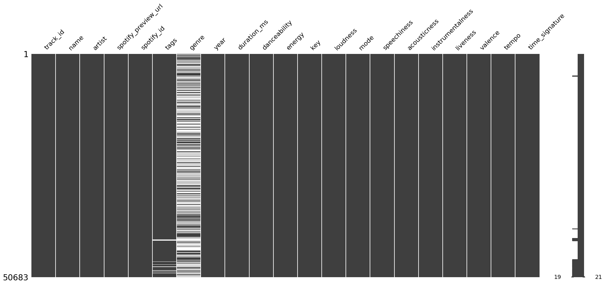
Only two columns, genre and tags, have missing values. We can see that genre has a lot of missing values. In fact, the majority of values (about 56%) in genre are missing, and they are missing at random. Further, tags has a lot fewer missing values (only about 2%).
Duplicates
We especially do not want duplicates in the data because the similarity score between duplicate songs will obviously be very high. We do not want duplicate songs as recommendations. Checking duplicates using the simple code
df_songs.duplicated().any()
gives False as the output. So, at first glance, it looks like we are good. However, when we checked for all songs with duplicate names using the following code
df_songs["name"].str.lower().duplicated().sum()
we found that a total of 815 songs had the same name. After printing these songs, we noticed that though the names are the same, the artists are different. So most of these songs are actually different.
To find duplicate songs in a better way, we added the condition that the songs are duplicates only if the values in the columns spotify_preview_url, spotify_id, artist, year, duration_ms, and tempo match. This is equivalent to running the following code.
df_songs.duplicated(subset=["spotify_preview_url", "spotify_id", "artist", "year", "duration_ms", "tempo"]).sum()
This gave 9 duplicate rows. We printed them, verified that they indeed are duplicate songs, and dropped them.
Column-wise Analysis
Firstly, for convenience and readability, we created a new column duration_mins using the column duraction_ms by running the following code:
df_songs["duration_mins"] = df_songs["duration_ms"].div(1000).div(60)
Next, we saved all the categorical columns in a list categorical_cols using the following code:
categorical_cols = df_songs.select_dtypes(include="object").columns
Next, we saved all the integer columns in a list integer_cols using the following code:
integer_cols = df_songs.select_dtypes(include="int").columns
Finally, we saved all the continuous columns in a list continuous_cols using the following code:
continuous_cols = df_songs.select_dtypes(include="float").columns
Further, we created the following function for categorical analysis on all the categorical columns:
def categorical_analysis(df, columns, k_artists=15):
    for column in columns:
        print(f"The column '{column}' has {df[column].str.lower().nunique()} categories.")

        if column in ["artist", "genre"]:
            print(df[column].value_counts().head(k_artists))

        if column == "genre":
            print(f"The unique categories in the column '{column}' are: {df[column].dropna().unique()}")

        print("#" * 150, end="\n\n")
This function gives the number of categories in each categorical column, and prints the top-15 value counts of the artist and genre columns.
We also created a function to do numerical analysis on all numerical columns, which is the following:
def numerical_analysis(df, columns):
    for column in columns:
        print(f"Numerical analysis for '{column}':", end="\n\n")
        print("Statistical summary:")
        print(df[column].describe(), end="\n\n")

        fig = plt.figure(figsize=(12, 4))
        plt.subplot(1, 2, 1)
        sns.histplot(df[column])
        plt.title(f"Histogram of '{column}'")

        plt.subplot(1, 2, 2)
        sns.boxplot(df[column])
        plt.title(f"Boxplot of '{column}'")
        plt.show();

        print("#" * 150, end="\n\n")

    print("Pairplot")
    sns.pairplot(df[columns])
    plt.show();
This function runs the describe method, plots a histogram and a box plot for each of the columns. At the end, it also plots a pair plot for all the columns.
All Categorical Columns
Running the function categorical_analysis on all the categorical columns, i.e., running the following code
categorical_analysis(df_songs, categorical_cols)
gave us the following result:
The column 'track_id' has 50674 categories.
######################################################################################################################################################
The column 'name' has 49860 categories.
######################################################################################################################################################
The column 'artist' has 8317 categories.
artist
The Rolling Stones 132
Radiohead 110
Autechre 105
Tom Waits 100
Bob Dylan 98
The Cure 94
Metallica 85
Johnny Cash 84
Nine Inch Nails 83
Sonic Youth 81
Elliott Smith 76
Iron Maiden 76
In Flames 76
Boards of Canada 75
Mogwai 75
Name: count, dtype: int64
######################################################################################################################################################
The column 'spotify_preview_url' has 50620 categories.
######################################################################################################################################################
The column 'spotify_id' has 50674 categories.
######################################################################################################################################################
The column 'tags' has 20054 categories.
######################################################################################################################################################
The column 'genre' has 15 categories.
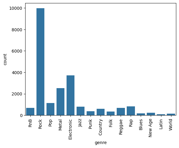
genre
Rock 9965
Electronic 3710
Metal 2516
Pop 1145
Rap 820
Jazz 793
RnB 696
Reggae 691
Country 607
Punk 383
Folk 355
New Age 237
Blues 189
World 140
Latin 100
Name: count, dtype: int64
The unique categories in the column 'genre' are: ['RnB' 'Rock' 'Pop' 'Metal' 'Electronic' 'Jazz' 'Punk' 'Country' 'Folk'
'Reggae' 'Rap' 'Blues' 'New Age' 'Latin' 'World']
######################################################################################################################################################
- The column
track_idhas all unique values. - The
nameof some songs are the same, which is understandable as names of two different songs can be the same. - These two columns also don’t help much for recommendations, the
track_iddue to its uniqueness, andnamedue to the fact that matching names does not imply similar songs. - The data consists of 8,317
artists, which can be used for recommendations since if people like a song from a particular artist, they may also like some other song by the same artist. - The column
spotify_preview_urlhas almost all values as unique. We won’t drop this column as it will be helpful in providing a preview audio of a song recommendation to users. - The column
spotify_idhas all its values unique. Again, this column won’t be helpful in giving recommendations due to its uniqueness. - The column
tagshas multple tags for the same song. We can use this column to use some vectorization technique. - The column
genrehas 15 categories. However this column also has about 56% of the values as missing.
genre
Recall that this column genre has a lot of missing values. Figure 3 shows the count plot of this column.
genre.To check if we can try to fill genre using the column tags, we grouped by genre and printed the genre and tags using the following code:
genre_group = df_songs.groupby("genre")
genre_group[["genre", "tags"]].sample(3)
We saw that the same genre can have different tags. Also, genre and tags are interchangeable in the data. Hence, it is not possible to fill the missing values in genre using tags.
Non-English name
Using the following code
df_songs.loc[df_songs.loc[:, "name"].str.contains("[^\d\w\s.?!':;-_(){},\.#-&/-]")]
we saw that there are about 39 rows for which the song name contains non-English characters. However, this is not a problem since we won’t be using the name of the song for recommendation purpose.
Non-English artist
Using the following code
df_songs.loc[df_songs.loc[:, "artist"].str.contains("[^\d\w\s.?!':;-_(){},\.#-&/-]")]
we saw that there are about 24 rows for which the artist name contains non-English characters. Again, this is not a problem as we will encode these later.
tags
Each row in the data has multiple values in the tags column. After adding all the tags in a set, we found that there are 100 unique tags in the entire data.
All Integer Columns
The integer columns we have are year, duration_ms, key, mode, and time_signature. Running the describe function on them gives the information shown in Table 6.
| year | duration_ms | key | mode | time_signature | |
|---|---|---|---|---|---|
| count | 50,674 | 50,674 | 50,674 | 50,674 | 50,674 |
| mean | 2004.02 | 251,153.64 | 5.31 | 0.63 | 3.90 |
| std | 8.86 | 107,589.21 | 3.57 | 0.48 | 0.42 |
| min | 1900 | 1,439 | 0 | 0 | 0 |
| 25% | 2001 | 192,733 | 2 | 0 | 4 |
| 50% | 2006 | 234,933 | 5 | 1 | 4 |
| 75% | 2009 | 288,183 | 9 | 1 | 4 |
| max | 2022 | 3,816,373 | 11 | 1 | 5 |
Table 6: Descriptive statistics for integer columns (values formatted for readability).
We can see that
- Most of the songs in the data seem to be after the year 2006.
- Most of the songs are in the time signature of 4.
Next, we ran the following code on the integer columns:
for col in integer_cols:
    print(f"The column '{col}' has {df_songs[col].nunique()} unique values.")
The output we got is the following:
The column 'year' has 75 unique values.
The column 'duration_ms' has 24202 unique values.
The column 'key' has 12 unique values.
The column 'mode' has 2 unique values.
The column 'time_signature' has 5 unique values.
Next, we ran the following code on the integer columns:
for col in integer_cols:
    print(f"The top category in the column '{col}' is:")
    print(f"{df_songs[col].value_counts().head(1)}", end="\n\n")
The output we got is the following:
The top category in the column 'year' is:
year
2007    4221
Name: count, dtype: int64

The top category in the column 'duration_ms' is:
duration_ms
214666    21
Name: count, dtype: int64

The top category in the column 'key' is:
key
9    5907
Name: count, dtype: int64

The top category in the column 'mode' is:
mode
1    31979
Name: count, dtype: int64

The top category in the column 'time_signature' is:
time_signature
4    44981
Name: count, dtype: int64
year
Figure 4 shows the histogram of the column year.
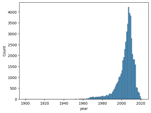
year.We can see that most of the songs are from the 2000’s.
key
Figure 5 shows the bar plot of the % value counts of the column key.
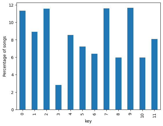
key.The key distribution seems random. However, the least number of songs are in the key 3, i.e., D♯.
mode
Figure 6 shows the count plot of the column mode.
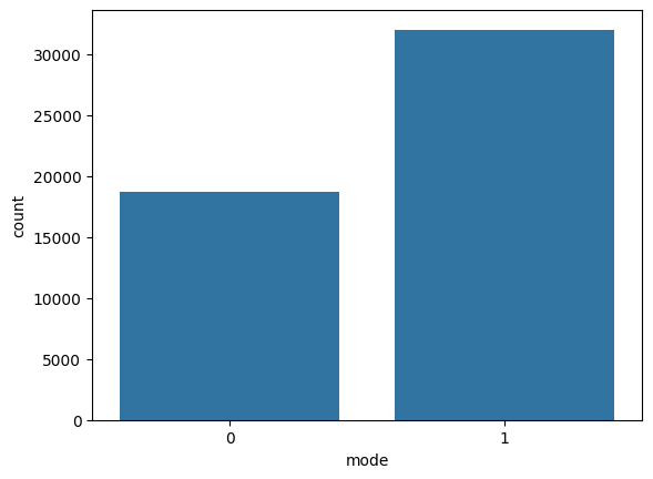
mode.We can see that most of the songs are in a major scale.
time_signature
Figure 7 shows the count plot of the column time_signature.
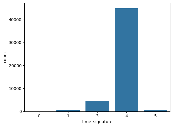
time_signature.We can see that the overwhelming majority of the songs hav a time signature of 4, and a very tiny fraction of songs have it as 0, 1, and 5.
duration_mins
Figure 8 shows the histogram of the column duration_mins.
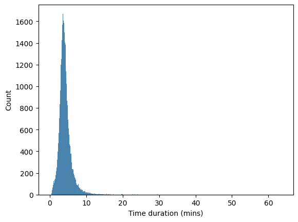
duration_mins.We can see that
- Vast majority of songs are between 1 to 10 minutes long.
- Duration has a long right tail, i.e., it is considerably right-skewed.
- This means that it has many outliers.
Figure 9 shows the box plot of this column.
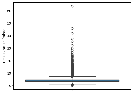
duration_mins.We can see that there is one song which is longer than 60 mins. We also printed this particular row. The song is legit.
All Continuous Columns
We ran the numerical_analysis function on all continuous columns using the following code:
numerical_analysis(df_songs, continuous_cols)
The output we got is the following.
danceability
The output of the describe method on danceability is the following:
Statistical summary:
count    50674.000000
mean         0.493522
std          0.178833
min          0.000000
25%          0.364000
50%          0.497000
75%          0.621000
max          0.986000
Name: danceability, dtype: float64
Further, the histogram and the box plot is shown in Figure 10.
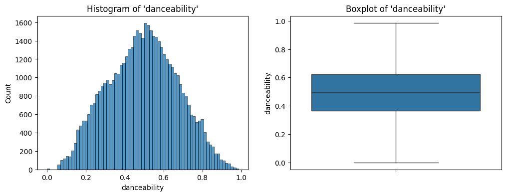
danceability.The distribution peaks at a danceability of 0.5, and seems symmetric.
energy
The output of the describe method on energy is the following:
Statistical summary:
count    50674.000000
mean         0.686507
std          0.251803
min          0.000000
25%          0.514000
50%          0.744000
75%          0.905000
max          1.000000
Name: energy, dtype: float64
Further, the histogram and the box plot is shown in Figure 11.
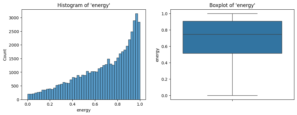
energy.The distribution looks left skewed with most songs having a high amount of energy.
loudness
The output of the describe method on loudness is the following:
Statistical summary:
count    50674.000000
mean        -8.291007
std          4.548359
min        -60.000000
25%        -10.375000
50%         -7.199500
75%         -5.089000
max          3.642000
Name: loudness, dtype: float64
Further, the histogram and the box plot is shown in Figure 12.
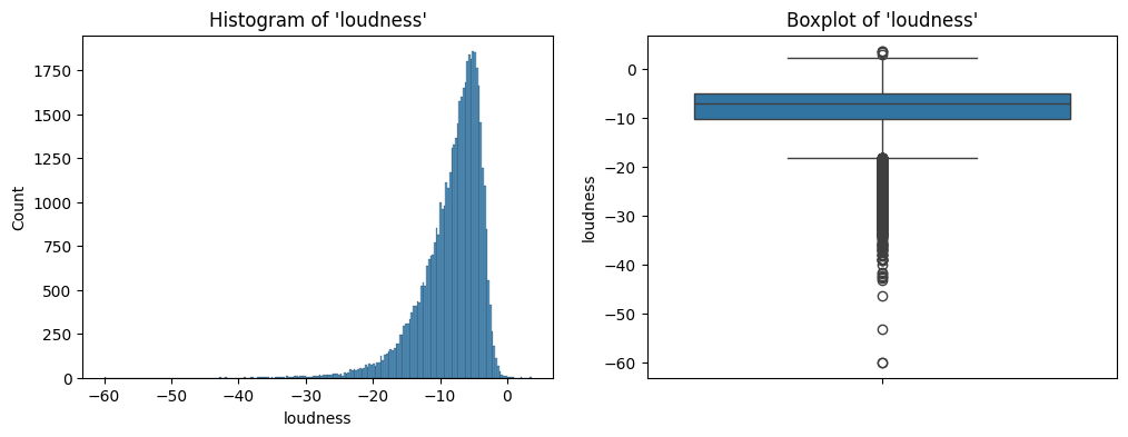
loudness.The distribution is extremely left skewed with most songs having a high value of loudness. There are also some extreme values that have a very low value of loudness.
speechiness
The output of the describe method on speechiness is the following:
Statistical summary:
count    50674.000000
mean         0.076026
std          0.076012
min          0.000000
25%          0.035200
50%          0.048200
75%          0.083500
max          0.954000
Name: speechiness, dtype: float64
Further, the histogram and the box plot is shown in Figure 13.
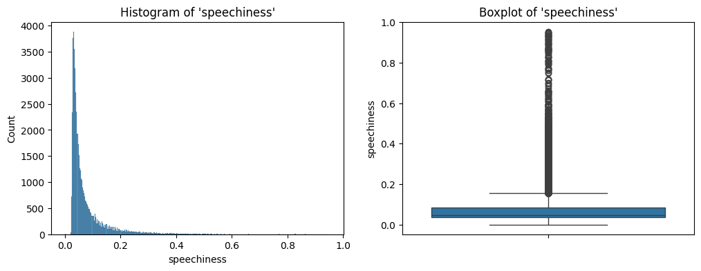
speechiness.The distribution is extremely right skewed with a lot of extreme values. Seems like our data has a lot of instrumental songs without any, or very less, vocals.
acousticness
The output of the describe method on acousticness is the following:
Statistical summary:
count    50674.000000
mean         0.213798
std          0.302839
min          0.000000
25%          0.001400
50%          0.039900
75%          0.340000
max          0.996000
Name: acousticness, dtype: float64
Further, the histogram and the box plot is shown in Figure 14.
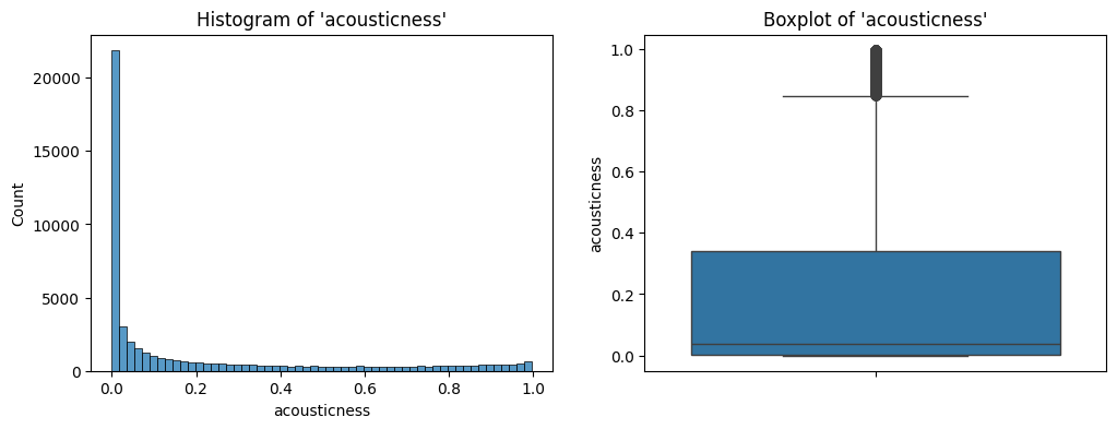
acousticness.The distribution is right skewed with extreme values. Looks like our data has most songs that are not acoustic.
instrumentalness
The output of the describe method on instrumentalness is the following:
Statistical summary:
count    50674.000000
mean         0.225299
std          0.337067
min          0.000000
25%          0.000018
50%          0.005630
75%          0.441000
max          0.999000
Name: instrumentalness, dtype: float64
Further, the histogram and the box plot is shown in Figure 15.
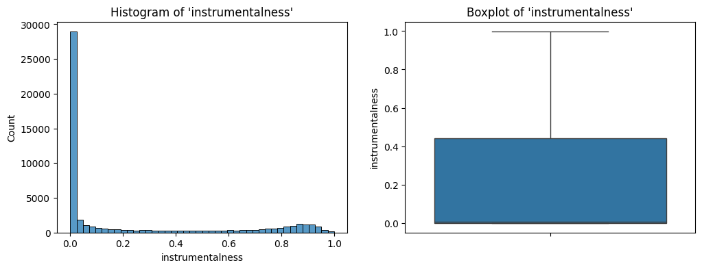
instrumentalness.The distribution is right skewed. Most songs have low value of instrumentalness.
liveness
The output of the describe method on liveness is the following:
Statistical summary:
count    50674.000000
mean         0.215439
std          0.184708
min          0.000000
25%          0.098400
50%          0.138000
75%          0.289000
max          0.999000
Name: liveness, dtype: float64
Further, the histogram and the box plot is shown in Figure 16.
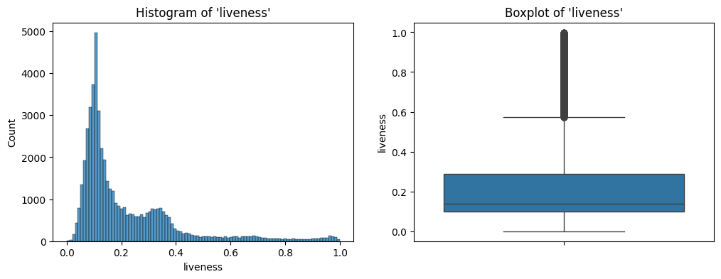
liveness.The distribution is a bit peculiar. It is bimodal with right skew. Most songs have low liveness, but there is a small peak at an intermediate value.
valence
The output of the describe method on valence is the following:
Statistical summary:
count    50674.000000
mean         0.433113
std          0.258767
min          0.000000
25%          0.214000
50%          0.405000
75%          0.634000
max          0.993000
Name: valence, dtype: float64
Further, the histogram and the box plot is shown in Figure 17.
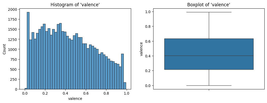
valence.The distribution looks close to uniform at for small values of valence, however it has a slight right skew at the end.
tempo
The output of the describe method on tempo is the following:
Statistical summary:
count    50674.000000
mean       123.508794
std         29.622349
min          0.000000
25%        100.682500
50%        121.989000
75%        141.642250
max        238.895000
Name: tempo, dtype: float64
Further, the histogram and the box plot is shown in Figure 18.
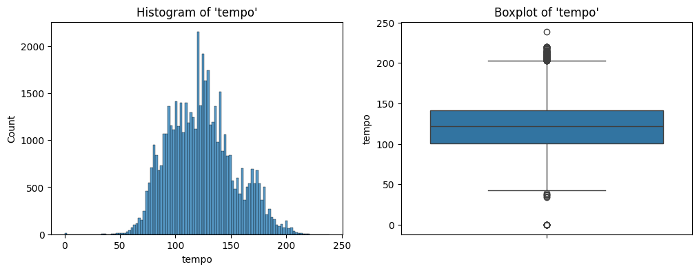
tempo.The distribution looks close to normal with extreme values in both directions.
duration_mins
The output of the describe method on duration_mins is the following:
Statistical summary:
count    50674.000000
mean         4.185893
std          1.793154
min          0.023983
25%          3.212217
50%          3.915550
75%          4.803046
max         63.606217
Name: duration_mins, dtype: float64
Further, the histogram and the box plot is shown in Figure 19.
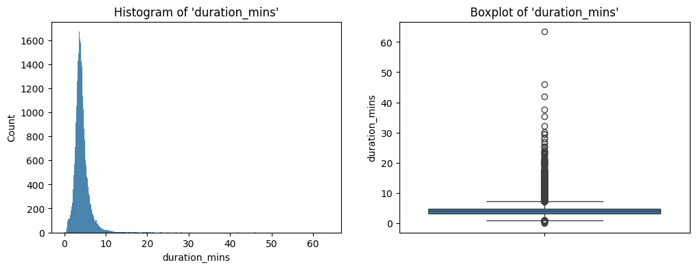
duration_mins.We have already seen these two plots before.
Pair Plot
The pair plot of all the continuous columns is shown in Figure 20.
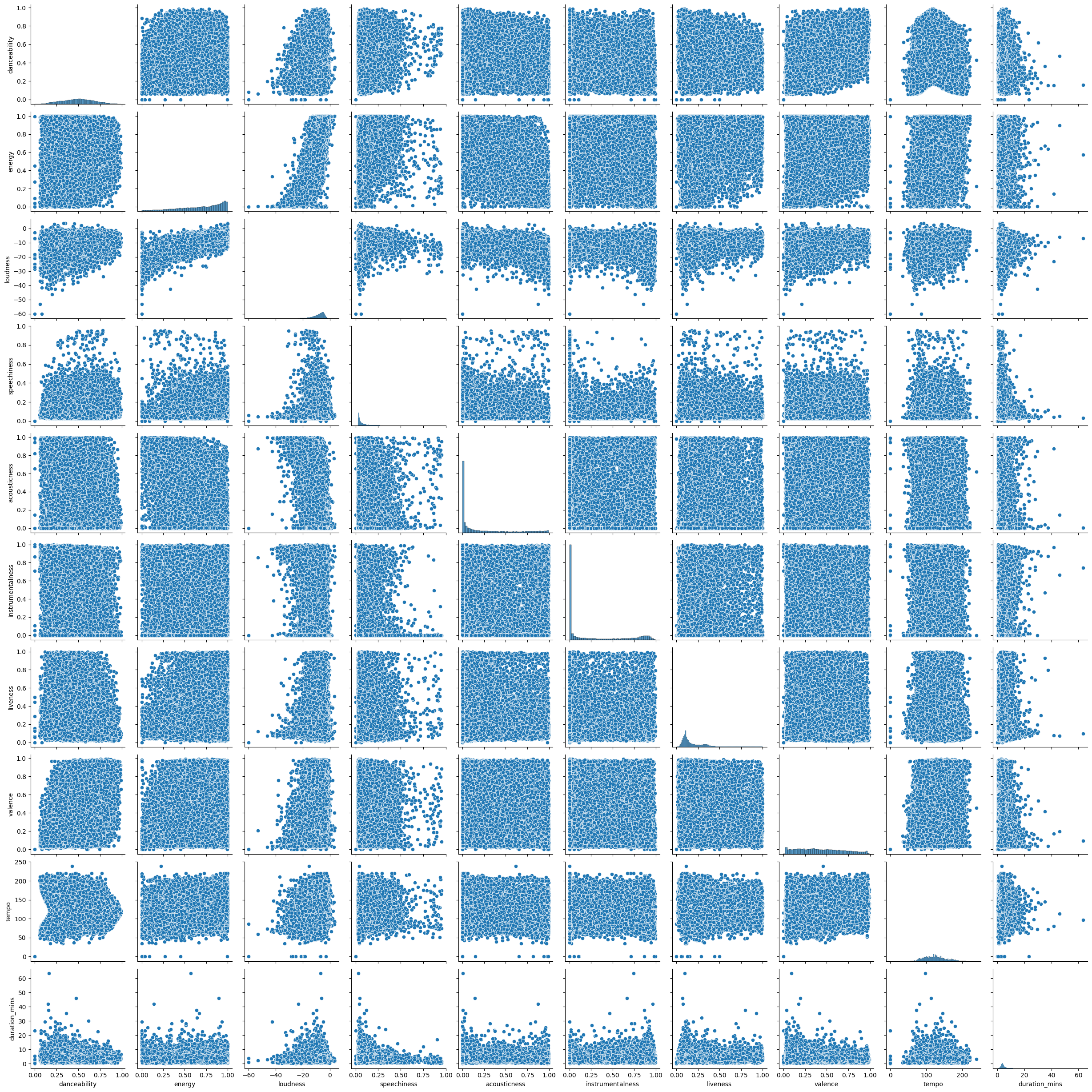
We can see that loudness and energy are positively correlated, i.e., if one increases, the other increases too. The same is true for danceability and loudness. The other columns do not seem to have any relationship.
User-Song Interaction Dataset
The description of this data is shown in Table 5. Fortunately, there are no duplicates and missing values in this data. Further, we also found that the number of unique users in this data is 962,037, and the number of unique songs are 30,459. The number of unique songs in the songs data is 50,683. This means that there are about 20 thousand or so songs that the users in this dataset have never heard.
We figured out the track_id’s for the songs that were played the most by the users using the following code:
df_users["track_id"].value_counts(sort=True).head(10)
Further, we viewed these songs in the songs dataset using the following code:
top_10_most_played_songs = df_users["track_id"].value_counts(sort=True).head(10)
df_songs.loc[df_songs["track_id"].isin(top_10_most_played_songs.index.tolist()), :]
Further, we found the songs with the highest play count using the following code:
df_users.groupby("track_id")["playcount"].agg("sum").sort_values(ascending=False)
We figured out that the songs that were played the most and the songs with the highest play count were almost the same. This was done using the following code:
top_10_most_played_songs_playcounts = df_users.groupby("track_id")["playcount"].agg("sum").sort_values(ascending=False).head(10)
pd.concat([top_10_most_played_songs, top_10_most_played_songs_playcounts], axis=1)
The most diverse users were found using the following code:
top_10_most_diverse_users = df_users.groupby("user_id")["track_id"].agg("count").sort_values(ascending=False).head(10)
These are the users that have played the most number of different songs. Further, we also found the most active users using the following code:
top_10_most_active_users = df_users.groupby("user_id")["playcount"].agg("sum").sort_values(ascending=False).head(10)
These are the users that have the highest play count. Concatenating both these types of users using the following code
pd.concat([top_10_most_diverse_users, top_10_most_active_users], axis=1)
we figured out that both these types of users are not the same. It looks like the most diverse users do not play the same song repeatedly, and hence have a relatively lower value of play count. Further, the most active users tend to play the same songs over and over again, making them have a high value of play count.
Jupyter Notebook
The entire EDA was performed in a Jupyter notebook which can be checked out here.
Content-Based Filtering Recommender System
As discussed before, we will first build a recommender system using content-based filtering. We will only be using the songs dataset here. In short, we will find the similarity matrix containing the similarity of each song with every other song. When the user plays a song, we will simply recommend the user the most similar songs to the song they have chosen to play.
Flow
We have about 50 thousand songs in the songs dataset. However, the issue with the data is the following. 56% of values in the genre column are missing. It is also not possible to fill the values using the tags column. Hence, we will drop the genre column.
The flow is the following:
- Drop the duplicates,
- Drop the
genrecolumn as it has most of its values as missing, - Fill the missing values in
tagscolumn with the value"no tags", - Convert all the text in the rows to lowercase,
- Get the data ready for content-based filtering:
- Decide on the features based on which the similarity will be calculated. For instance, columns like
name, ID-based columns, etc., are unique for every song. Hence, we will drop these so that they don’t interfere while calculating the similarity. Specifically, we drop the columnstrack_id,name,spotify_preview_url, andspotify_id.
- Decide on the features based on which the similarity will be calculated. For instance, columns like
- Apply transformations on the data to vectorize (or numerically encode) it,
- Calculate the similarity using cosine similarity,
- Recommend the user top-\(k\) most similar songs to what they are listening to right now.
Building the System in Jupyter Notebook
We will first build the entire content-based filtering recommender system in a Jupyter notebook, and then copy the code to Python modules which will be later included as a part of a DVC pipeline. We follow the same steps as listed above.
Data Transformation
The transformation techniques (encoding and scaling) and the respective columns they are applied on are listed in Table 7.
| Transformation Technique | Applied Columns |
|---|---|
Frequency Encoding | year |
One-hot Encoding | artisttime_signaturekey |
TF-IDF | tags |
Standard Scaling | duration_msloudnesstempo |
Min-max Scaling | danceabilityenergyspeechinessacousticnessinstrumentalnesslivenessvalence |
Table 7: Transformation techniques and the columns they are applied to.
These were applied using scikit-learn’s ColumnTransformer. The code for this is the following:
freq_enc_cols = ["year"]
ohe_cols = ["artist", "time_signature", "key"]
tfidf_col = "tags"
std_scaler_cols = ["duration_ms", "loudness", "tempo"]
min_max_scaler_cols = [
    "danceability",
    "energy",
    "speechiness",
    "acousticness",
    "instrumentalness",
    "liveness",
    "valence"
]

transformer = ColumnTransformer(
    transformers=[
        (
            "frequency_encoder",
            CountEncoder(normalize=True, return_df=True),
            freq_enc_cols
        ),
        ("one_hot_encoder", OneHotEncoder(handle_unknown="ignore"), ohe_cols),
        ("tfidf", TfidfVectorizer(max_features=85), tfidf_col),
        ("standard_scaler", StandardScaler(), std_scaler_cols),
        ("min_max_scaler", MinMaxScaler(), min_max_scaler_cols),
    ],
    remainder="passthrough",
    n_jobs=-1,
    force_int_remainder_cols=False,
)
This transformer was fitted on the data and was used to transform the same.
Finding Most Similar Songs
We first pick the song “Whenever, Wherever” by the artist “Shakira” from the original data and consider it as the input. In other words, we will find the similarity of this song with all the songs in the data. We first pick the row corresponding to this song, transform it using the trained ColumnTransformer object defined above and find the cosine similarity using the function cosine_similarity from scikit-learn. This gives us a matrix of shape (50674, 1), which is understandable as we have a total of 50,674 songs in the data, and this matrix consists of the similarity score of the song “Whenever, Wherever” with all the songs. Next, using the argsort function from NumPy, we find the indices of the songs that are the most similar, and print those rows from the data.
We also create a function that does this entire job, which is the following:
def recommend(song_name, songs_data, transformed_data, k=10):
    song_row = songs_data.loc[songs_data["name"] == song_name, :]
    if song_row.empty:
        print(f"Song '{song_name}' is not present in the data.")
    else:
        song_index = song_row.index[0]
        print(f"Song index: {song_index}")
        input_vector = transformed_data[song_index].reshape(1, -1)
        similarity_scores = cosine_similarity(transformed_data, input_vector)
        print(f"similarity_scores.shape: {similarity_scores.shape}")
        top_k_most_similar_songs_idxs = np.argsort(similarity_scores.ravel())[::-1][1:][:k]
        print(f"Similarity scores of the {k} songs that are most similar to the song '{song_name}': {top_k_most_similar_songs_idxs}")
        top_k_most_similar_songs_name = songs_data.loc[top_k_most_similar_songs_idxs]
        top_k_most_similar_songs_list = top_k_most_similar_songs_name[["name", "artist", "spotify_preview_url"]].reset_index(drop=True)
        return top_k_most_similar_songs_list
Jupyter Notebook
The Jupyter notebook in which all of this was done can be checked out here.
Building the System in a DVC Pipeline
The stages in the DVC pipeline are the following:
Data Cleaning
The following steps are carried out in this stage:
- Loading the raw songs data,
- Dropping duplicates,
- Dropping unnecessary columns,
- Filling missing values,
- Converting entries in some columns to lowercase,
- Saving the cleaned data.
This is implemented in the content_based_filtering/data_cleaning module, which can be checked out here.
Data Preparation
The following steps are carried out in this stage:
- Loading the cleaned data that was saved in the previous stage,
- Dropping columns not needed to find similarity,
- Saving the prepared data.
This is implemented in the content_based_filtering/data_preparation module, which can be checked out here.
Data Transformation
The following steps are carried out in this stage:
- Loading the prepared data that was saved in the previous stage,
- Creating the
ColumnTransformerobject to encode features, - Training the
ColumnTransformerobject, - Transforming the prepared data,
- Saving the transformed data and the trained
ColumnTransformerobject.
This is implemented in the content_based_filtering/data_transformation module, which can be checked out here.
Recommendation using Content-Based Filtering
The following steps are carried out in this stage:
- Loading the cleaned data and the transformed data,
- Taking a song name from the cleaned data as input,
- Getting the corresponding row of this song from the transformed data,
- Finding the similarity score of this song (transformed) with all the songs (transformed),
- Finding and printing the top-\(k\) most similar songs to this input song.
This is implemented in the content_based_filtering/recommendation module, which can be checked out here.
dvc.yaml
All these stages are combined in a DVC pipeline using dvc.yaml file, which can be checked out here. Running the command
dvc repro
from the root directory of the terminal, i.e., the directory which contains this dvc.yaml file, will run the DVC pipeline.
Streamlit App
A Streamlit app was also built that gives recommendations based on content-based filtering. The app does the following:
- Loads the cleaned songs data,
- Loads the transformed (or vectorized) songs data,
- Takes the song name as input from the user and the number of recommendations the user wants,
- Gets recommendations using the
Recommenderobject of thecontent_based_filtering/recommendationmodule, - Displays the current song the user is listening to (i.e., the input song) and the recommendations.
This is implemented in the app.py module, which can be checked out here. Running the command
streamlit run app.py
starts the app.
Collaborative Filtering Recommender System
Now, we will build a recommender system using only collaborative filtering by using the user-song interaction data. As the number of users (962,037) in the data is a lot more as compared to the number of items or songs (30,459), we will be building an item-based collaborative filtering system. In other words, we will create an item-user (song-user in this case) interaction matrix in which each row will correspond to a song and each column will correspond to a user. Further, each entry in this matrix will stand for the playcount, i.e., the number of times that particular song is played by the corresponding user. Next, we will choose a random song, i.e., a random row of this matrix, as the input song and find its similarity with all the songs in the matrix, i.e., all the rows. Finally, we will show the users the top-\(k\) similar songs to this input song.
Issue
There is an issue, which is the fact that if we create the item-user interaction matrix, then it will have a shape of \(30459 \times 962037\), which means that it will have a whopping \(29302684983\) (close to 30 billion) entries. Even if each entry takes 2 bytes of space, the total space needed to store this matrix will be 60 billion bytes, or 60 GBs. We do not have this much RAM to store this matrix. Further, this matrix will be sparse as almost all users will be such that they would have listened to only a tiny subset of these 30,459 songs.
This is a huge bottleneck. To solve this, we will use the Python library Dask. It is designed to work with large datasets using chunking. The operations on each chunk are performed in parallel.
Why Dask?
Dask has many advantages. Some of them are the following:
- It is very similar to
pandasandNumPy. More specifically, they have very similar methods. Hence learning is easy. - It has support for parallel processing that use cores on a multi-core CPU or multiple clusters on platforms like Kubernetes.
- It handles big data by dividing it into manageable sized chunks.
- It has wrappers over many other frameworks like machine learning algorithms in
scikit-learn, deep learning algorithms inkeras/torch, boosting, etc. So,Daskworks with all these algorithms by parallelizing their training on large datasets.
Working of Dask
Dask has multiple objects defined that are collectively called collections. We are only concerned with the Dask.DataFrame collection. There are also other collections like Dask.Array
Dask has the following three main components:
- Client: This is the component that interacts with the user. Whenever the user writes some
pandas/NumPy-like code usingDask, the client converts the operations in the code into task graphs. - Scheduler: The scheduler understands the task graph created by the client and checks which operations can be parallelized and assigns these tasks to the workers.
- Worker: These can be nodes on a cluster or cores on a multi-core CPU.
Dask stores these task graphs and does not execute the functions or transformations indicated in them unless the compute method is called. Once this method is called, the transformations are carried out parallely on the chunks.
Flow
The flow of building the item-based collaborative filtering recommender system is the following:
- Convert the indices of the unique users and unique songs to integer,
- Creating the item-user (song-user) interaction matrix using
Dask, - Converting this matrix into a sparse matrix to save space,
- Calculate similarity using cosine similarity,
- Recommender the user top-\(k\) most similar songs to what they are listening to right now.
Building the System in Jupyter Notebook
Again, we will first build the entire item-based collaborative filtering recommender system in a Jupyter notebook, and then copy the code to Python modules which will be later included as a part of a DVC pipeline. We will follow the same steps as listed above.
Creating the Item-User Interaction Matrix
Using the user-song interaction dataset, we have found all the unique tracks (or songs) by running the unique method on the track_id column. Next, we have filtered the songs dataset to get the details of these particular songs only. So, right now we have the songs dataset that contain information about the songs (i.e., their attributes like the artist name, danceability, liveness, etc.) and the user-song interaction dataset that contains the songs, the user ID, and the playcount. Both these dataset have information of the same common songs.
Next, we need to create the item-user interaction matrix. As mentioned before, each row of this matrix will correspond to a particular song (track_id), each column will correspond to a particular user (user_id), and each entry will be the number of times that song is played by the corresponding user (playcount). To save space, we need to encode the row and the column indices into integers. We do this using the categorize method of Dask.DataFrame. We will store these encoded indices in the user-song interaction data as new columns.
So, earlier this data had three columns, track_id, user_id, and playcount (see Table 5). After creating these new indices as new columns, the data now has the columns track_id, user_id, playcount, track_idx, and user_idx. Now, we will group by the columns track_idx and user_idx and use the sum aggregate function on the playcount column. This will give us the information about which user has played which song for how many times. Using this we will create the item-user interaction matrix, which will be a sparse matrix.
Jupyter Notebook
The Jupyter notebook in which all these steps were carried out can be checked out here.
Building the System in a DVC Pipeline
The new stages added in the DVC pipeline are the following:
Data Filtering
The following steps are carried out in this stage:
- Loading the cleaned songs data and the user-song interaction data,
- Getting the unique track IDs from the user-song interaction data,
- Filtering the songs data to only include tracks present in the user-song interaction data.
This is implemented in the collaborative_filtering/data_filtering module, which can be checked out here.
Interaction Matrix
The following steps are carried out in this stage:
- Loading the user-song interaction data,
- Converting the
playcountcolumn to float, - Creating the new integer indices as new columns for the user IDs and the track IDs,
- Saving the newly created track IDs,
- Creating the item-user interaction (sparse) matrix,
- Saving the item-user interaction matrix.
This is implemented in the collaborative_filtering/interaction_matrix module, which can be checked out here.
Recommendation using Collaborative Filtering
The following steps are carried out in this stage:
- Loading the filtered songs data, the track IDs (that were saved in the previous stage), and the interaction matrix (that was saved in the previous stage),
- Getting the input song and the input artist,
- Getting the index of this input song,
- Getting the corresponding row of this input song from the interaction matrix using the index,
- Calculating the similarity of the input song with all the songs,
- Getting the top-\(k\) most similar songs to the input songs.
This is implemented in the collaborative_filtering/recommendation module, which can be checked out here.
Updated dvc.yaml
All these new stages are added and combined in the same DVC pipeline using the same dvc.yaml file, which can be checked out here. Again, running the
dvc repro
command from the root directory of the terminal, i.e., the directory which contains this dvc.yaml file, will run the DVC pipeline.
Streamlit App
We now make changes in the already existing app.py module to include collaborative filtering. For now, we will give the user the option to choose the recommendation method, i.e., content-based filtering or collaborative filtering. The steps for content-based filtering are the same as before. With respect to collaborative filtering, new steps are added in this module, which are the following
- Loading the cleaned songs data (this step is common between content-based and collaborative filtering),
- Loading the filtered songs data,
- Getting the collaborative filtering recommendations using the
Recommenderobject from thecollaborative_filtering/recommendationmodule.
The code for UI is the same as before. The updated app.py module can be checked out here. Running the command
streamlit run app.py
starts the app.
Hybrid Recommender System
We will now combine the recommendations given by content-based and collaborative filtering recommender systems using a weighted approach. What gets weighted are the similarity scores of both these methods. Let \(w_{\text{cb}}\) denote the weight of content-based filtering method and \(w_{\text{cf}}\) denote the weight of collaborative filtering method. Then, the similarity scores of the hybrid recommender system are given by
\[\begin{multline}\label{eq:hybrid_weighted_approach} (\text{similarity scores})_{\text{hybrid}} = w_{\text{cb}} \times (\text{similarity scores})_{\text{cb}}\\+ w_{\text{cf}} \times (\text{similarity scores})_{\text{cf}}, \end{multline}\]such that
\[\begin{equation*} w_{\text{cb}} + w_{\text{cf}} = 1. \end{equation*}\]A clear problem that is visible here is that if we use the original songs data to find similarity scores for content-based filtering system, we will get an array of shape \(50683\times 1\). This is because there are 50,683 songs in that data. Further, for the collaborative filtering sytem, we have to use the filtered songs data, which has 30,459 songs. This means that the similarity scores array of shape \(30459\times 1\) for the collaborative filtering system. As the dimensions of both these arrays do not match, we won’t be able to use Equation \eqref{eq:hybrid_weighted_approach}. So, we will need to use the filtered songs data only to build the hybrid recommender system so that the linear combination of both the similarity scores arrays is possible. For now, we will keep the values of the weights as the following: \(w_{\text{cb}} = 0.3\), and \(w_{\text{cf}} = 0.7\). We will change these later and dynamically update the weights depending on the user. However, there are still two major problems in this system. Let us discuss them.
Problems
Mismatch in Index Positions
The index positions of the songs in the similarity scores array of content-based filtering and collaborative filtering do not match. Hence, directly taking the linear combination between them would be wrong. It would be like adding apples to oranges. The reason why this problem arises is because the ordering of rows in the filtered songs data used for content-based filtering is not the same as the order of the rows in the interaction matrix used for collaborative filtering. Recall that we built the interaction matrix by using the categorize method. This method assigns indices by first lexicographically sorting the column based on which the index is to be formed (which is the column track_id in our case). However, the filtered songs data used for content-based filtering is not sorted based on the track_id column.
Solution
The solution is simple. Before using the filtered songs data for content-based filtering, we will first sort it based on the column track_id and then transform it to calculate the similarity scores. This will make sure that the index order the similarity scores array for content-based filtering and the similarity scores array for collaborative filteirng are the same. This will allow us to take their linear combination.
Difference in the Scale of Similarity Scores
The similarity scores of the content-based filtering system are significantly closer to \(1\) as compared to collaborative filtering system. This is because the interaction matrix used in the latter is a sparse matrix. The cosine similarity between sparse vectors results in a smaller value as compared ot non-sparse vectors. This makes the recommender system biased for content-based filtering, which is a problem.
Solution
Again, the solution is simple. We will separately normalize (using min-max scaling) the similarity scores arrays before taking their linear combination.
Building the System in a DVC Pipeline
Instead of building it in Jupyter notebook first, we will directly build it in a DVC pipeline. The new stages added in the DVC pipeline are the following:
Feature Preparation
The following steps are carried out in this stage:
- Loading the collab-filtered songs CSV and sorting it by
track_id, - Loading the already-trained content-based filtering transformer,
- Transforming the sorted songs to produce a sparse feature matrix,
- Saving the sorted CSV and the aligned sparse feature matrix for hybrid use.
This is implemented in the hybrid_recommendation/feature_preparation module, which can be checked out here.
Recommendation using Hybrid Approach
The following steps are carried out in this stage:
- Loading the collaborative filtering universe (track IDs + interaction matrix) and the content-based filtering features aligned to the collab-filtered songs (sorted by
track_id), - Computing cosine similarities for both content-based filtering and collaborative filtering for the seed item,
- Normalizing each similarity vector (min-max) to mitigate scale differences,
- Reindexing collaborative filtering similarities to the songs DataFrame order, ensuring 1:1 alignment,
- Combining (element-wise) using weights \(w_{\text{cb}}\) and \(w_{\text{cf}}\), excludes the seed, and returns top-\(k\).
This is implemented in the hybrid_recommendation/recommendation module, which can be checked out here.
Updated dvc.yaml
All these new stages are added and combined in the same DVC pipeline using the same dvc.yaml file, which can be checked out here. Again, running the
dvc repro
command from the root directory of the terminal, i.e., the directory which contains this dvc.yaml file, will run the DVC pipeline.
Streamlit App
Another method for hybrid recommender system, called handle_hybrid, was added in the streamlit app code, i.e., in the app.py module. It uses the recommend method of the Recommender class from the hybrid_recommendation/recommendation module. In the UI, we also added a slider to choose the weight \(w_{\text{cbf}}\). Once this weight is choosen by the user, it automatically selects the value for the weight \(w_{\text{cf}}\) such that
The updated app.py module can be checked out here. Running the command
streamlit run app.py
starts the app.
Improving the Hybrid Recommender System
There are some problems with our recommender system. Let us discuss them one by one.
Cold Start Problem
To understand this problem better, let us recall what we have done with respect to the data so far. When we built the content-based filtering system, we considered the songs data which contained attributes of 50,683 songs. When we built the collaborative filtering system, we considered the user-song interaction data which contained 30,459 unique songs. Finally, when we built the hybrid recommender system, we considered only these 30,459 songs that are common between the songs data and the user-song interaction data as we could not apply collaborative filtering on the remaining 20,224 songs since we did not have their playcounts. However, this is not a very good idea as it accounts to a significant proportion of all the songs we have.
To solve this problem, we will do the following. We will consider these 20,224 songs to be new songs that no user has listened to yet. So if a user searches for a song among these, we won’t be able to give them any recommendation using the collaborative filtering component of the hybrid recommendation system. This is called the cold start problem. This problem arises when a user searches for a new song that no one has listened to before.
To solve this problem, we will do the following. If a user searches for a song that is present in the 30,459 common songs between both the datasets, then we will use the hybrid recommendation model to give them recommendations. However if they search for a song among the 20,224 new songs in the data that no one has listened to before, we will only use content-based filtering to provide recommendations.
Repeated Loading of Data
This is a problem with our Streamlit code. Every time the “Get Recommendations!” button is clicked, the data is loaded again, which is inefficient. To solve this problem, we will be saving the data in streamlit.session_state such that the data is cached. Now, the data is only loaded once when the app is started and stored in streamlit.session_state. When the “Get Recommendations!” button is clicked, only the similarity score is calculated and the recommendations based on this score are displayed. This significantly improves the speed of our application.
Both of these problems were addressed and fixed in the latest app.py code.
Evaluation Metrics
There are some advanced metrics that can be used to evaluate recommender systems. However, since we do not have labeled data (i.e., data about whether the given recommendations were useful to the user), we won’t be able to use them. But we will still discuss them.
Precision@\(k\)
Precision@\(k\) is given by
\[\begin{equation}\label{eq:precision_at_k} \mathrm{Precision@}k = \frac{\text{Number of relevant items in top-$k$}}{k}. \end{equation}\]For instance, say the number of recommendations given to a user are \(3\) (i.e., \(k = 3\)), and the following are the ground truth and the prediction:
- Ground truth: Item 1, Item 2, Item 4.
- Prediction: Item 2, Item 4, Item 5.
We can see that items 2 and 4 are common. These are the relevant items. So, precision@\(3\), using Equation \eqref{eq:precision_at_k}, is given by
\[\begin{equation*} \mathrm{Precision@}k = \frac{2}{3}. \end{equation*}\]Precision can be thought of as the accuracy, or quality, of the recommendations.
Recall@\(k\)
Recall@\(k\) is given by
\[\begin{equation}\label{eq:recall_at_k} \mathrm{Recall@}k = \frac{\text{Number of relevant items in top-$k$}}{\text{Total number of relevant items}}. \end{equation}\]Model-Based Recommender System
We will briefly talk about model-based recommender systems. These recommender systems are generally applied using collaborative filtering. A popular method is using singular value decomposition (SVD).
Singular Value Decomposition (SVD)
Recall that the user-song interaction data had the columns track_id, user_id, and playcount. It basically had the information about how many times a particular user played a particular song. Now what happens in SVD is that we take the unique values in track_id and build latent features. These latent features are hidden features about the tracks. SVD gives the following decomposition of the data:
Here, the matrix \(\mathbf{U}\) has the rows as the track_id values and the columns as its latent features. The rows of the matrix \(\mathbf{V}\) has rows as the user_id values, and the columns will be the latent features. Finally, the matrix \(\mathbf{\Sigma}\) is a diagonal matrix, where the values on the diagonal will tell us the importance of the latent features. It tells us which user_id and track_id pair is more relevant based on which we can carry out the prediction.
The prediction works in the following way. The item-user interaction matrix, which in our case is the song-user interaction matrix, is sparse. The rows in this matrix correspond to songs and the columns correspond to users. Each entry corresponds to how many times that particular user has played that particular song. In collaborative filtering, we have to recommend those songs to a particular user that they haven’t played yet based on the similarity of either songs or users. The model focuses on the songs that the user has not played yet and predicts their playcount. It finally recommends those songs to the user that has the highest value of this prediction. So, the model actually converts the sparse interaction matrix into a dense matrix by making predictions.
The metrics used are the same as the ones used in regression problems, like mean absolute error, mean squared error, root mean squared error, etc. We can train the model to improve these metrics.
Towards Deployment
We want to deploy the Streamlit app. This app needs the following data:
- Songs data,
- Transformed (or encoded) version of the songs data,
- The array of track IDs,
- Interaction matrix,
- Filtered songs data,
- Transformed version of the filtered songs data.
All these datasets are being tracked using DVC. The flow for the future steps leading to deployment are the following:
- Continuous Integration (CI):
- We will run the app on a GitHub runner and perform certain tests.
- Continuous Delivery (CD):
- We will containerize the app into a Docker container by creating a Docker image.
- We will push this Docker image to Amazon ECR.
- We will pull this image and run the app on a single Amazon EC2 instance. We will do this manually.
- Deployment:
- We will use CodeDeploy to deploy the app using the blue-green deployment strategy.
- We will do this by creating an auto-scaling group with a minimum capacity of 2 and a maximum capacity of 5. This will also be the deployment group.
We will be using the version of the Docker image to keep track of the versions of app in deployment. These versions will be mentioned in the tags and will be maintained on ECR.
Continuous Integration (CI)
Our data is already tracked by DVC. We will now simply create a workflow file and add the following steps in it:
- Code checkout:
- This step will copy the code on the GitHub repository on to the GitHub runner.
- Installing Python and required libraries:
- This step will install Python and all the libraries required to run the app.
- Authenticate using AWS S3:
- This step will help the runner authenticate with AWS S3 so that it can communicate with the S3 bucket where the required data is stored.
- Pulling the data on to the runner from S3:
- This step will pull all the data required by the app to run from S3 on to the runner.
- Starting the app on the runner:
- We will now start the Streamlit app on the runner.
- Test the endpoint:
- Once the app starts, we will test whether we are able to access the endpoint of this app.
Workflow File
We will now create a new file ci-cd.yaml inside the .github/workflows directory in the root directory of the project. This file will contain all the commands and instructions to run the code and tests on the GitHub runner. This file contains the following code:
name: CI-CD

on: push

jobs:
  CI-CD:
    runs-on: ubuntu-latest
    steps:
      - name: Code Checkout
        uses: actions/checkout@v4

      - name: Setup Python
        uses: actions/setup-python@v5
        with:
          python-version: '3.12.0'
          cache: 'pip'

      - name: Install Packages
        run: |
          python -m pip install --upgrade pip
          pip install -r requirements.txt

      - name: Configure AWS Credentials
        uses: aws-actions/configure-aws-credentials@v4
        with:
          aws-access-key-id: ${{ secrets.AWS_ACCESS_KEY_ID }}
          aws-secret-access-key: ${{ secrets.AWS_SECRET_ACCESS_KEY }}
          aws-region: us-east-2

      - name: DVC Pull
        run: |
          dvc pull

      - name: Run Appllication
        run: |
          nohup streamlit run app.py --server.port 8000 &
          sleep 30

      - name: Test App
        run: |
          pytest tests/test_app.py

      - name: Stop Streamlit app
        run: |
          pkill -f "streamlit run"
Before pushing this code onto the GitHub repository to run this on the runner, we will create two secrets, AWS_ACCESS_KEY_ID and AWS_SECRET_ACCESS_KEY, inside the repository.
Test
We will carry out a simple test of checking whether the home page of the app is loading or not. This is in the tests/test_app.py module, which can be found here. The simple code in this module is th efollowing:
import requests
import time

APP_URL = "http://localhost:8000"


# Getting the status code
def get_app_status(url):
    response = requests.get(url)
    status_code = response.status_code
    return status_code


# Testing for the app home page loading
def test_app_loading():
    # Waiting for the app to load
    time.sleep(60)
    status_code = get_app_status(APP_URL)
    assert status_code == 200, "Unable to load Streamlit App"
    print("Streamlit App Loaded Successfully")
It simply checks whether the app is loading correctly by checking whether the status code is 200 or not. Once this test is carried out and is successful, the streamlit app is closed and the CI workflow ends.
Continuous Delivery
Creating the Docker Image
We will now create a Docker image of our app, run it locally, and test it. To create the Docker image, we create a Dockerfile in the project root that contains instructions on how to do so. The instructions in it will be the following:
- Installing Python:
- We don’t actually install Python. Instead, we use an image of Python that is already present on DockerHub. This will be the base image.
- Setting the working directory:
- This is the directory, or the root folder, relative to which all the paths in the Docker image are defined.
- Copying the requirements file:
- This amounts to copying all requirements file that contains all the packages needed to run the Streamlit app.
- We will also run the
pip install requirements.txtcommand once the file is copied.
- Copying the required datasets:
- This amounts to copying all the datasets that will be used by the Streamlit app to make predictions.
- Copying the required Python modules:
- This step will copy all the Python modules required to run the app.
- Exposing a port:
- Now a port will be exposed that will be used to communicate with the app. This port will be
8000.
- Now a port will be exposed that will be used to communicate with the app. This port will be
- Running the Streamlit app:
- This will be the command that will run the Streamlit app.
All these steps are translated inside the Dockerfile in the following way:
FROM python:3.12

WORKDIR /app

COPY requirements-dev.txt .
RUN pip install -r requirements-dev.txt

COPY data/interim/Music_Info_cleaned.csv            data/interim/
COPY data/interim/collab_filtered_songs.csv         data/interim/
COPY data/interim/collab_filtered_songs_sorted.csv  data/interim/
COPY data/processed/Music_Info_cleaned_transformed_CBF.npz data/processed/
COPY data/processed/collab_track_ids.npy            data/processed/
COPY data/processed/collab_interaction_matrix.npz   data/processed/
COPY data/processed/hybrid_transformed_cbf.npz      data/processed/

COPY spotify_recommender/__init__.py                               spotify_recommender/
COPY spotify_recommender/config.py                                 spotify_recommender/
COPY spotify_recommender/content_based_filtering/__init__.py       spotify_recommender/content_based_filtering/
COPY spotify_recommender/content_based_filtering/recommendation.py spotify_recommender/content_based_filtering/
COPY spotify_recommender/collaborative_filtering/__init__.py       spotify_recommender/collaborative_filtering/
COPY spotify_recommender/collaborative_filtering/recommendation.py spotify_recommender/collaborative_filtering/
COPY spotify_recommender/hybrid_recommendation/__init__.py         spotify_recommender/hybrid_recommendation/
COPY spotify_recommender/hybrid_recommendation/recommendation.py   spotify_recommender/hybrid_recommendation/

COPY app.py .

EXPOSE 8000
CMD ["streamlit", "run", "app.py", "--server.port", "8000", "--server.address", "0.0.0.0"]
This will result in the following structure of the working directory inside the container:
/               # Root of the container
├─ app/         # Working directory
│  ├─ data/
│  │  ├─ interim/
│  │  │  ├─ collab_filtered_songs.csv
│  │  │  ├─ collab_filtered_songs_sorted.csv
│  │  │  ├─ Music_Info_cleaned.csv
│  │  ├─ processed/
│  │  │  ├─ collab_interaction_matrix.npz
│  │  │  ├─ collab_track_ids.npy
│  │  │  ├─ hybrid_transformed_cbf.npz
│  │  │  ├─ Music_Info_cleaned_transformed_CBF.npz
│  ├─ spotify_recommender/
│  │  ├─ collaborative_filtering/
│  │  │  ├─ recommendation.py
│  │  ├─ content_based_filtering/
│  │  │  ├─ recommendation.py
│  │  ├─ hybrid_recommendation/
│  │  │  ├─ recommendation.py
│  │  ├─ config.py
│  ├─ app.py
Now, running the command
docker build -t spotify_recommender:v0.1.0 .
builds this Docker image. Notice how we carrying out versioning using the tags. Once the image is built, running the command
docker run --name spotify_recommender -d -p 8000:8000 spotify_recommender:v0.1.0
runs the docker container. We ran the container and checked that it was working correctly.
Pushing the Image to Amazon ECR
We will now build, tag, and push the image to Amazon ECR using the GitHub runner. We will use the same ci-cd.yaml workflow file to do this.
We first create a new repository on Amazon ECR and then add the following new steps in this workflow file:
      - name: Configure AWS Credentials
        uses: aws-actions/configure-aws-credentials@v4
        with:
          aws-access-key-id: ${{ secrets.AWS_ACCESS_KEY_ID }}
          aws-secret-access-key: ${{ secrets.AWS_SECRET_ACCESS_KEY }}
          aws-region: us-east-2

      - name: Log in to Amazon ECR
        id: login-ecr
        uses: aws-actions/amazon-ecr-login@v2

      - name: Build, Tag, and Push Docker Image to Amazon ECR
        env:
          REGISTRY: ${{ steps.login-ecr.outputs.registry }}
          REPOSITORY: ${{ secrets.ECR_REPOSITORY_URI }}
          IMAGE_TAG: latest
        run: |
          docker build -t $REGISTRY/$REPOSITORY:$IMAGE_TAG .
          docker push $REGISTRY/$REPOSITORY:$IMAGE_TAG
Once we push the code to GitHub, this workflow is triggered and the image is pushed to Amazon ECR. Once the image was pushed, we also manually pulled the image onto our local machine and checked if it was running correctly.
Deployment on AWS
Manual Deployment on a Single EC2 Instance
Now we will use the image on ECR and launch it manually on a single Amazon EC2 instance. We will follow these steps:
- Launch the EC2 instance.
- Install Docker in the instance.
- Install AWS CLI version 2.
- Authenticate with AWS using the command
aws configure. - Connect the Docker service with ECR.
- Pull the image on the EC2 instance.
- Run the container on the EC2 instance.
Steps 1 to 3
Before launching the EC2 instance, we need to create an IAM role that will handle the communication between ECR and the EC2 instance. This role will help pull the image that is right now on ECR. The trusted entity type for this role is AWS service, and the use case is EC2. The permissions policy added to this role is the AmazonEC2ContainerRegistryFullAccess.
Now, we will manually launch an EC2 instance. This will be a t2.micro instance with Ubuntu and the appropriate rules in the security group. Once we connect to this instance and open the terminal, we run the following commands in it:
sudo apt-get update -y

sudo apt-get install -y docker.io

sudo systemctl start docker
sudo systemctl enable docker

sudo usermod -aG docker ubuntu

sudo apt-get install -y unzip curl

curl "https://awscli.amazonaws.com/awscli-exe-linux-x86_64.zip" -o "/home/ubuntu/awscliv2.zip"
unzip -o /home/ubuntu/awscliv2.zip -d /home/ubuntu/
sudo /home/ubuntu/aws/install

rm -rf /home/ubuntu/awscliv2.zip /home/ubuntu/aws
These commands do the following:
- Update the package lists.
- Install Docker.
- Start and enable Docker service.
- Add “ubuntu” user to the “docker” group to run Docker commands without
sudo. - Install necessary utilities.
- Download and install AWS CLI version 2.
- Clean up the AWS CLI installation files.
Authentication with AWS
Now, we will simply run the
aws configure
command and enter the required keys to authenticate with AWS.
Authenticating and Connecting the Docker service with ECR
This simply amounts to running the first push command of the repository on present on the ECR.
Pulling the image on the EC2 instance
This simply amounts to running the last push command of the ECR repository (the one with docker push...), with push replaced by pull. We will also rename the image using the docker tag command to the shorter name “spotify_recommender” and add the tag “latest” to it.
Running the container on the EC2 instance
We will run the container using the following command:
docker run -d --name spotify_recommender -p 8000:8000 spotify_recommender:latest
Accessing the Container
By visiting on the public IP with the port 8000, we confirmed that the container was running correctly and the recommendations were correct.
Blue-Green Deployment
🚧 Work in Progress: This page is currently being written. Some sections are complete, while others are still under construction. Feel free to explore and check back later for updates!