flowchart TD
    A["Linear models fit only straight lines"] --> B["Feature maps: x becomes ϕ(x)"]
    B --> C["LMS with features: just plug in ϕ(x)"]
    C --> D["Problem: ϕ(x) blows up to about d³"]
    D --> E["Insight: θ is always a combo of the data"]
    E --> F["Rewrite the algorithm with a kernel K(x, z)"]
    F --> G["ϕ vanishes: the kernelized algorithm"]
    G --> H["Kernels as similarity: choose K directly"]
    H --> I["Payoff: the 14 houses, fit"]
    I --> J["Which K are legal? Mercer, and closure rules"]
    J --> K["The reach of the kernel trick; on to SVMs"]

    style D fill:#c0392b,color:#fff
    style F fill:#2471a3,color:#fff
    style G fill:#1e8449,color:#fff
    style I fill:#1e8449,color:#fff
Kernel Methods
Machine Learning
Supervised Learning
Mathematics
A first-principles tour of kernel methods: from feature maps and polynomial regression, through the kernel trick that hides an infinite-dimensional feature space behind a cheap function, to Mercer’s theorem, the closure rules that let you build kernels from kernels, and the reach of the kernel idea.
Where We Left Off
In the linear regression post, we built our very first supervised learning algorithm: fit a straight line (or a flat hyperplane) to data. It was simple, it had a clean closed-form solution, and it worked. But it carried a quiet limitation that we mostly glossed over: it can only ever fit straight things. A line for one input, a plane for two, a flat hyperplane for many. Real relationships curve.
We did sneak in one escape hatch. To fit a curved trend, we can invent new inputs, like \(x^2\) and \(x^3\), and hand those to the same old linear machinery. The fit looks curved in the original variable even though the model is still linear in the (expanded) inputs. That trick was powerful, but it left an awkward question hanging in the air: how many new inputs should we add? Ten? A thousand? Could we, in some wild fantasy, add infinitely many?
This post takes that fantasy seriously. We will see that with an idea called the kernel trick, we really can work in feature spaces so enormous, even infinite-dimensional, that we could never write down a single feature vector on a computer, and yet still train and predict efficiently. Along the way, the humble inner product will turn out to be the secret hero of the whole story.
This post is largely based on the treatment in Ng & Ma (2023) and the accompanying lecture (Stanford Online, Anand Avati, 2019). Where a deeper or alternative treatment helps, we lean on the standard references Hastie et al. (2009), Bishop (2006), and the kernel-methods monograph Schölkopf & Smola (2002).
A concrete itch: a curve a line cannot fit
Let us make the limitation concrete. Suppose we are predicting the price \(y\) of a house from a single number \(x\), its living area. We collect fourteen houses and plot them, with area measured in thousands of square feet and price in hundreds of thousands of dollars. The trend is real but it is not straight: prices climb steeply across the small homes, flatten out through the middle of the market where an extra bedroom barely moves the number, and then climb again at the luxury end. Figure 1 shows what happens when we try to fit it.
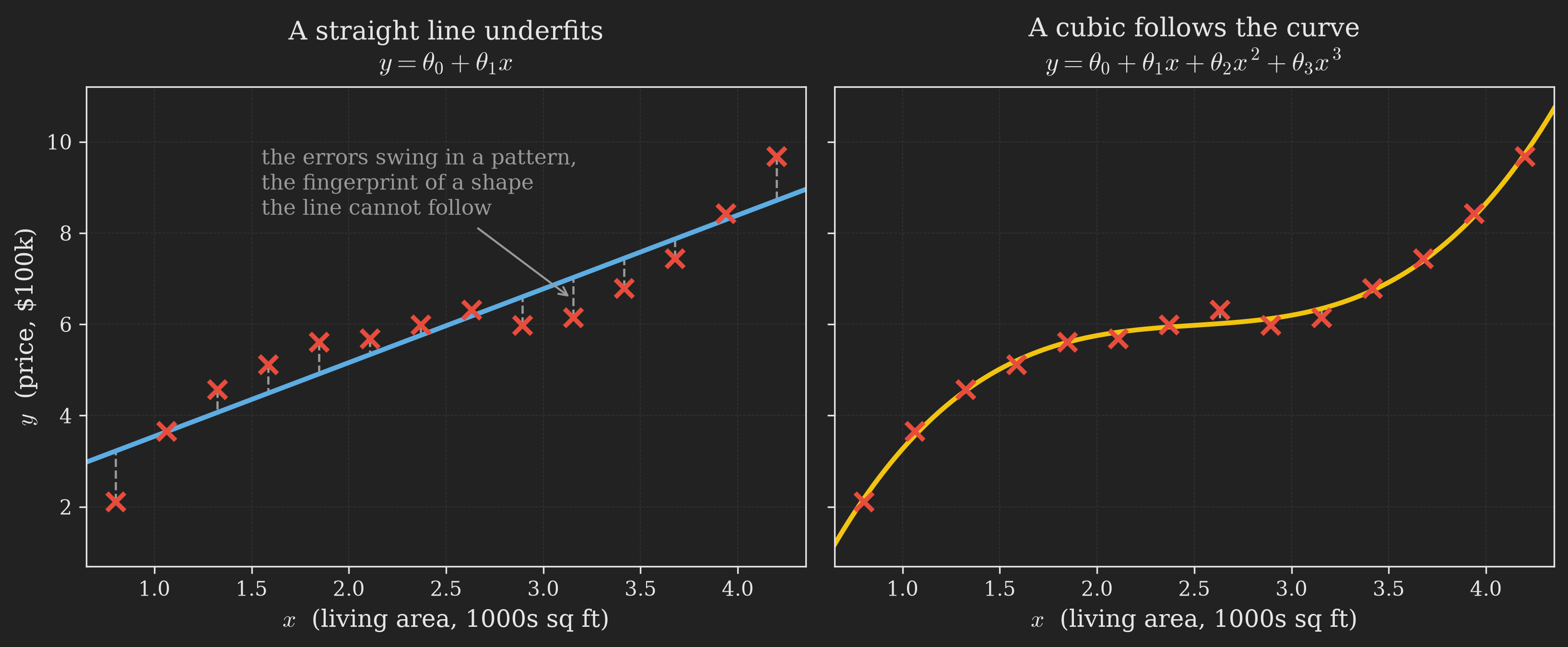
Look at the dashed residual segments on the left. They are not scattered randomly around the line, which is what honest noise would look like; they swing in a systematic arc. That signature is the tell-tale sign of a model that is missing real structure, not just unlucky. The cubic on the right absorbs that structure. So how do we fit that cubic using the linear regression we already know? That is where our journey begins.
These same fourteen houses will follow us through the whole post. By the end we will fit them with a feature space we never write down.
The roadmap
Before we set off, here is the whole trail on one map. We start from the “add polynomial features” idea, watch it run into a computational wall, and then discover the kernel trick that tears the wall down. Figure 2 sketches the path.
Four boxes are highlighted because they are the emotional beats of the story: the red one (the wall), the blue one (the trick that gets us past it), and the two green ones (the trick paying off, first in principle and then on our actual fourteen houses). Keep them in the back of your mind.
Feature Maps
Let us formalize the “invent new inputs” idea. Fitting a cubic
\[ y = \theta_3 x^3 + \theta_2 x^2 + \theta_1 x + \theta_0 \]
feels nonlinear, but watch what happens if we bundle the powers of \(x\) into a single vector. Define a function \(\boldsymbol{\upphi} : \mathbb{R} \to \mathbb{R}^4\) by
\[ \boldsymbol{\upphi}(x) = \begin{bmatrix} 1 \\ x \\ x^2 \\ x^3 \end{bmatrix} \in \mathbb{R}^4, \tag{1}\]
and collect the coefficients into \(\boldsymbol{\uptheta} \in \mathbb{R}^4\), where
\[ \boldsymbol{\uptheta} = \begin{bmatrix} \theta_0 \\ \theta_1 \\ \theta_2 \\ \theta_3 \end{bmatrix}. \]
Then the cubic is just a dot product:
\[ \theta_3 x^3 + \theta_2 x^2 + \theta_1 x + \theta_0 = \begin{bmatrix} \theta_0 & \theta_1 & \theta_2 & \theta_3 \end{bmatrix} \begin{bmatrix} 1 \\ x \\ x^2 \\ x^3 \end{bmatrix} = \boldsymbol{\uptheta}^{\intercal} \boldsymbol{\upphi}(x). \tag{2}\]
Read Equation 2 slowly, because it is the hinge of everything that follows. A cubic in \(x\) is a linear function of the new quantities \(\boldsymbol{\upphi}(x)\). The nonlinearity did not disappear; it got absorbed into the inputs. The model on top is as linear as ever.
This deserves some vocabulary, and it is vocabulary we will use for the rest of the post:
- The original input \(x\) (the living area) is called the attributes of the problem.
- The transformed quantities \(\boldsymbol{\upphi}(x) = \begin{bmatrix} 1 & x & x^2 & x^3 \end{bmatrix}^{\intercal}\) are called the features.
- The function \(\boldsymbol{\upphi}\) that turns attributes into features is called a feature map.
(Different authors sometimes swap these words around, so if you read elsewhere and the terminology feels flipped, do not panic. Within this post, attributes go in, features come out.)
Nothing forces the attributes to be one-dimensional. In general, a feature map is a function
\[ \boldsymbol{\upphi} : \mathbb{R}^d \to \mathbb{R}^p, \]
taking a \(d\)-dimensional attribute vector \(\vb{x}\) to a \(p\)-dimensional feature vector \(\boldsymbol{\upphi}(\vb{x})\). For the cubic example we had \(d = 1\) and \(p = 4\). In a moment we will let \(p\) get frighteningly large.
One small but important point about \(\boldsymbol{\upphi}\), because it trips people up later: a feature map takes exactly one input. When we start writing things like \(\boldsymbol{\upphi}(\vb{x})^{\intercal}\boldsymbol{\upphi}(\vb{z})\), that is the same function \(\boldsymbol{\upphi}\) applied separately to \(\vb{x}\) and to \(\vb{z}\), and then the two results dotted together. There is no such thing as “\(\boldsymbol{\upphi}\) of the pair \((\vb{x}, \vb{z})\).” Keep that straight and a lot of what follows will feel less slippery.
NoteAn intuition worth building: why higher dimensions help
Feature maps help with classification too, and there the payoff is easy to see. Imagine two classes in a plane: an inner blob near the origin and an outer ring around it (think of the blue and red points below). No straight line can separate them; a line always leaves some of the ring on the same side as the blob.
Now apply the feature map
\[ \boldsymbol{\upphi} \left( \begin{bmatrix} x_1\\ x_2 \end{bmatrix} \right) = \begin{bmatrix} x_1\\ x_2\\ x_1^2 + x_2^2 \end{bmatrix}, \]
which gives every point a third coordinate equal to its squared distance from the origin. The inner blob, being close to the origin, stays low; the outer ring shoots up. In this lifted 3D space a perfectly flat plane slides between the two classes. Figure 3 runs through exactly this lift, in five beats: a straight line spinning in the plane and failing at every angle, the lift itself, the separating plane appearing, an orbit to prove the separation is not a trick of the viewing angle, and finally the payoff.
That last beat is the one to watch. When the points sink back down, the plane leaves a shadow behind: a circle. The flat boundary upstairs and the curved boundary downstairs are the same boundary, seen from two different spaces. The feature map did not make the problem linear by straightening the data; it moved the data somewhere a straight cut could reach it.
The moral, which holds for regression just as much as classification: a well-chosen feature map can turn a problem that is hopeless for a linear model into one a linear model handles with ease. This is a sidebar to build intuition; our main derivation below stays with regression. If the picture already convinced you that “more features = more power,” you can carry that feeling forward and read on.
LMS With Features
Having a feature map is one thing; training with it is another. Happily, the training changes almost nothing. Recall from the linear regression post that the batch gradient descent update for ordinary least squares, fitting \(h_{\boldsymbol{\uptheta}}(\vb{x}) = \boldsymbol{\uptheta}^{\intercal}\vb{x}\), is
\[ \boldsymbol{\uptheta} := \boldsymbol{\uptheta} + \alpha \sum_{i=1}^{n} \left( y_i - \boldsymbol{\uptheta}^{\intercal} \vb{x}_i \right) \vb{x}_i, \tag{3}\]
where \(\alpha\) is the learning rate and the sum runs over all \(n\) training examples. To fit \(\boldsymbol{\uptheta}^{\intercal}\boldsymbol{\upphi}(\vb{x})\) instead, we do the laziest possible thing: replace every \(\vb{x}_i\) by its feature vector \(\boldsymbol{\upphi}(\vb{x}_i)\). The update becomes
\[ \boldsymbol{\uptheta} := \boldsymbol{\uptheta} + \alpha \sum_{i=1}^{n} \left( y_i - \boldsymbol{\uptheta}^{\intercal} \boldsymbol{\upphi}(\vb{x}_i) \right) \boldsymbol{\upphi}(\vb{x}_i). \tag{4}\]
The stochastic (one-example-at-a-time) version is the same idea with the sum stripped away:
\[ \boldsymbol{\uptheta} := \boldsymbol{\uptheta} + \alpha \left( y_i - \boldsymbol{\uptheta}^{\intercal} \boldsymbol{\upphi}(\vb{x}_i) \right) \boldsymbol{\upphi}(\vb{x}_i). \tag{5}\]
The only real difference between Equation 3 and Equation 4 hides in the dimensions. In ordinary least squares, \(\boldsymbol{\uptheta} \in \mathbb{R}^d\), one weight per attribute. With features, \(\boldsymbol{\uptheta} \in \mathbb{R}^p\), one weight per feature. As long as \(p\) is modest, we are done: this is a complete, working algorithm. The trouble starts when \(p\) is not modest.
When Features Explode
Here is where the story hits its wall. The cubic feature map for a single attribute was harmless: four features. But suppose our attributes are genuinely high-dimensional, \(\vb{x} \in \mathbb{R}^d\), and we want the model to see all interactions up to degree three. Then the feature vector must contain every monomial of degree at most three:
\[ \boldsymbol{\upphi}(\vb{x}) = \begin{bmatrix} 1 \\ x_1 \\ x_2 \\ \vdots \\ x_1^2 \\ x_1 x_2 \\ x_1 x_3 \\ \vdots \\ x_1^3 \\ x_1^2 x_2 \\ \vdots \end{bmatrix}. \tag{6}\]
Counting the constant, the \(d\) linear terms, the \(d^2\) quadratic terms, and the \(d^3\) cubic terms, the feature vector has about \(1 + d + d^2 + d^3\) entries, which is of order \(d^3\).
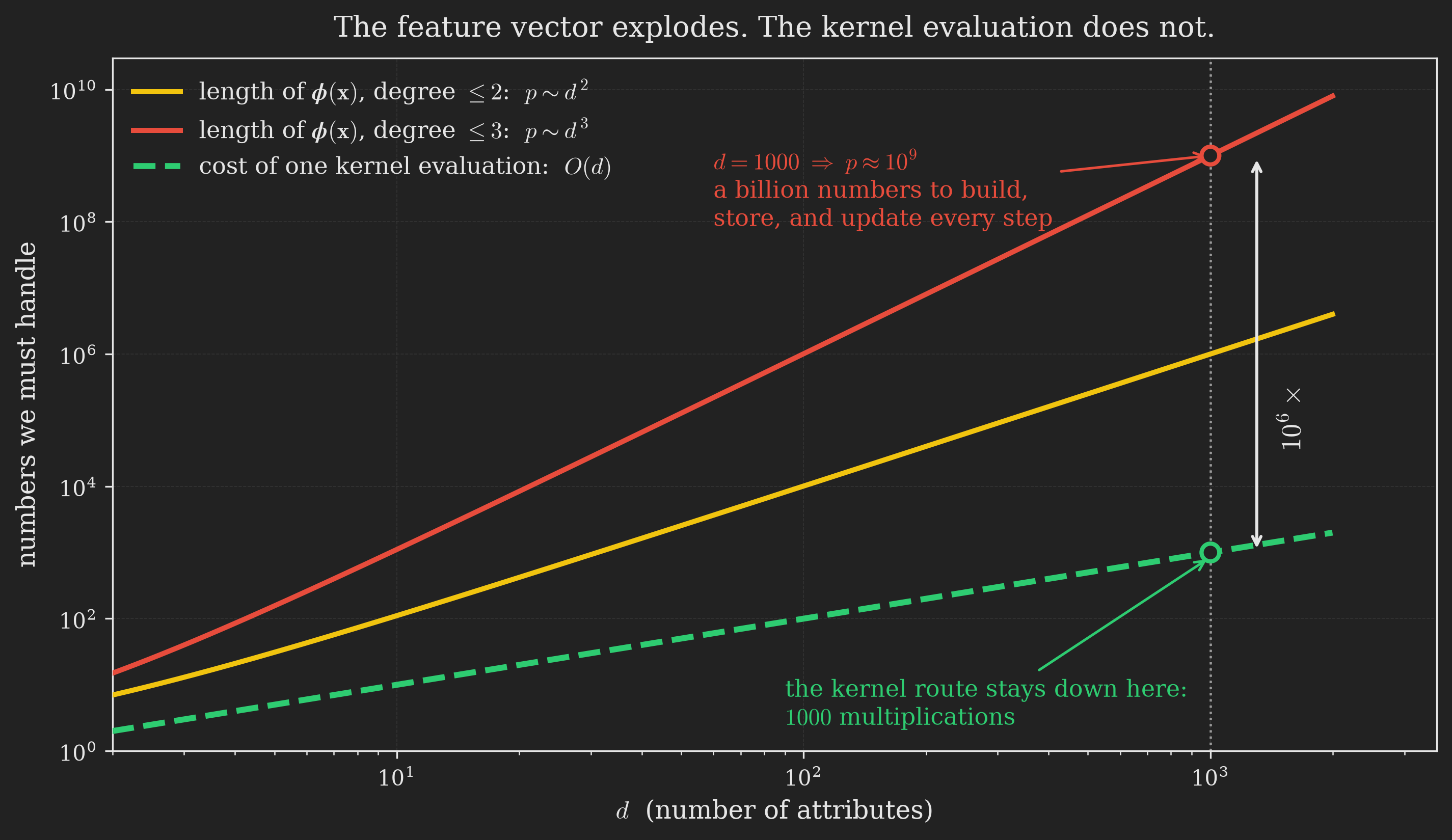
Let us feel how bad that is. Take \(d = 1000\), a perfectly ordinary size. Then \(p \approx d^3 = 10^9\). Every single gradient descent update in Equation 4 must build, store, and dot with vectors of a billion numbers. Compare that to ordinary least squares in Equation 3, where each update touches vectors of length \(d = 1000\). We just made every step roughly \(d^2 = 10^6\), a million, times slower, and we blew up our memory by the same factor. And all of that cost bought us nothing conceptually new; we merely chose a richer feature space.
Words like “a million times slower” are easy to read past, so Figure 4 draws the gap on a log scale. The dashed green line at the bottom is the target we will be aiming for by the end of this post.
It is tempting to conclude that this cost is simply unavoidable. After all, \(\boldsymbol{\uptheta}\) itself lives in \(\mathbb{R}^p\) with \(p \approx d^3\); surely we have to store all billion of its entries and update every one of them?
That intuition is exactly what the next three sections will demolish. The punchline, worth previewing so you know why we are about to do some algebra: we will never store \(\boldsymbol{\uptheta}\) at all.
The Kernel Trick, Step 1: \(\boldsymbol{\uptheta}\) Lives in the Span of the Data
The first crack in the wall is an observation so simple it is almost invisible. Suppose we start gradient descent from \(\boldsymbol{\uptheta} = \vb{0}\). Then at every iteration, \(\boldsymbol{\uptheta}\) is a linear combination of the feature vectors of the training points:
\[ \boldsymbol{\uptheta} = \sum_{i=1}^{n} \beta_i \, \boldsymbol{\upphi}(\vb{x}_i), \tag{7}\]
for some scalars \(\beta_1, \ldots, \beta_n\). Not one weight per feature, but one weight per training example.
Why is this true? By induction. At initialization, \(\boldsymbol{\uptheta} = \vb{0} = \sum_{i=1}^{n} 0 \cdot \boldsymbol{\upphi}(\vb{x}_i)\), so the claim holds with all \(\beta_i = 0\). Now suppose it holds at some step, that is, \(\boldsymbol{\uptheta} = \sum_{i=1}^{n} \beta_i \, \boldsymbol{\upphi}(\vb{x}_i)\). Plug this into the update Equation 4 and collect terms:
\[ \begin{align*} \boldsymbol{\uptheta} :=& \: \, \boldsymbol{\uptheta} + \alpha \sum_{i=1}^{n} \left( y_i - \boldsymbol{\uptheta}^{\intercal} \boldsymbol{\upphi}(\vb{x}_i) \right) \boldsymbol{\upphi}(\vb{x}_i) \\ =& \sum_{i=1}^{n} \beta_i \, \boldsymbol{\upphi}(\vb{x}_i) + \alpha \sum_{i=1}^{n} \left( y_i - \boldsymbol{\uptheta}^{\intercal} \boldsymbol{\upphi}(\vb{x}_i) \right) \boldsymbol{\upphi}(\vb{x}_i) \\ =& \sum_{i=1}^{n} \underbrace{\left( \beta_i + \alpha \left( y_i - \boldsymbol{\uptheta}^{\intercal} \boldsymbol{\upphi}(\vb{x}_i) \right) \right)}_{\text{new } \beta_i} \boldsymbol{\upphi}(\vb{x}_i). \end{align*} \]
The updated \(\boldsymbol{\uptheta}\) is again a linear combination of the same \(n\) feature vectors, just with new coefficients. The induction goes through. So no matter how gigantic \(p\) is, and no matter how long we run gradient descent, \(\boldsymbol{\uptheta}\) never escapes the span of the \(n\) feature vectors \(\boldsymbol{\upphi}(\vb{x}_1), \ldots, \boldsymbol{\upphi}(\vb{x}_n)\).
It is worth pausing on what this means geometrically, because the algebra above hides a rather beautiful picture. The feature space \(\mathbb{R}^p\) is enormous. But the \(n\) feature vectors \(\boldsymbol{\upphi}(\vb{x}_1), \ldots, \boldsymbol{\upphi}(\vb{x}_n)\) span a slice of it that is at most \(n\)-dimensional, and what we just proved is that \(\boldsymbol{\uptheta}\) starts inside that slice and every gradient step keeps it there. The parameter is not free to roam \(\mathbb{R}^p\); it is confined to a low-dimensional plane pinned down entirely by the training data. Figure 5 draws it.
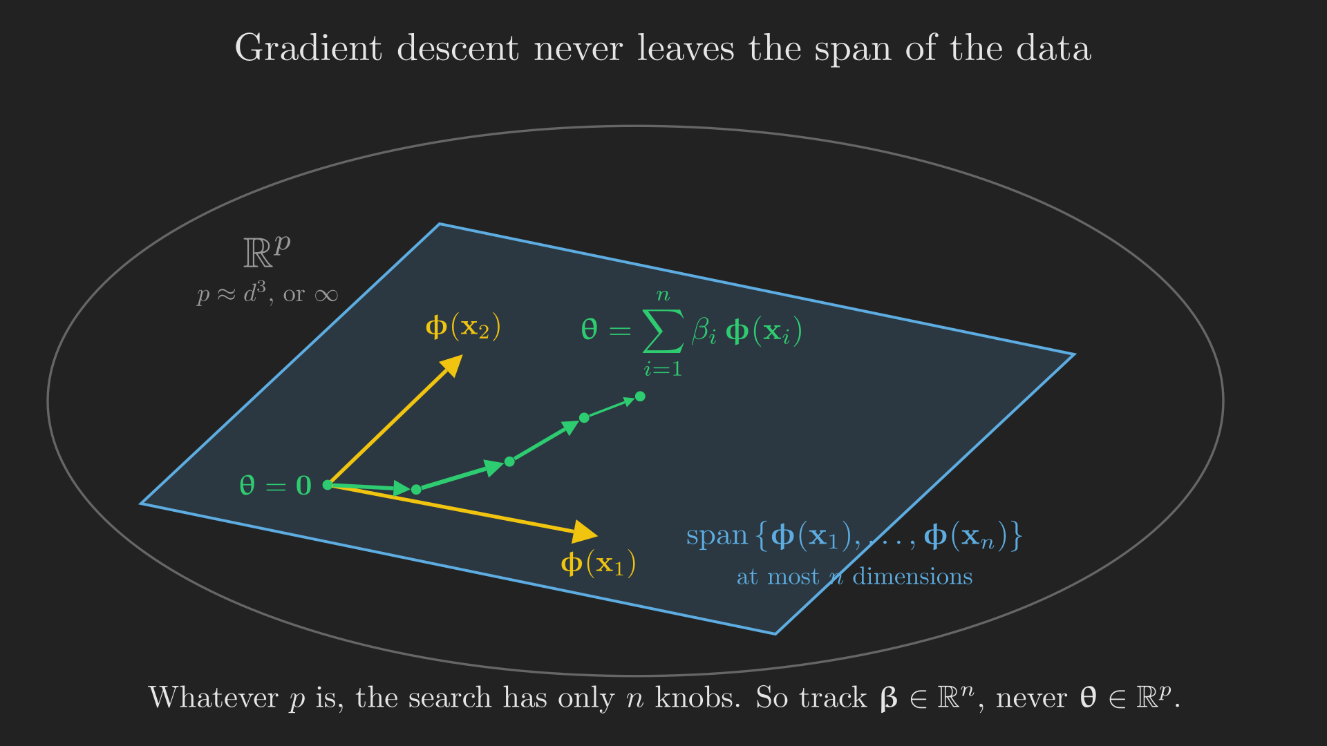
This suggests a change of bookkeeping. Instead of tracking the \(p\)-dimensional vector \(\boldsymbol{\uptheta}\), track the \(n\) coefficients \(\boldsymbol{\upbeta} = \begin{bmatrix} \beta_1 & \cdots & \beta_n \end{bmatrix}^{\intercal}\). Same model, different address: \(\boldsymbol{\uptheta}\) gives one weight per feature and can be endlessly long, while \(\boldsymbol{\upbeta}\) gives one weight per training example and is exactly as long as your dataset.
This is our first genuine win. We have traded a potentially infinite object for a finite one. But a nagging worry remains: the update for the new \(\beta_i\) still mentions the old \(\boldsymbol{\uptheta}\) through the term \(\boldsymbol{\uptheta}^{\intercal}\boldsymbol{\upphi}(\vb{x}_i)\). We have not actually gotten rid of \(\boldsymbol{\uptheta}\) yet; we have only promised to. Let us make good on the promise.
The Kernel Trick, Step 2: Rewrite Everything With the \(\beta\)’s
From the induction above, the coefficient update is
\[ \beta_i := \beta_i + \alpha \left( y_i - \boldsymbol{\uptheta}^{\intercal} \boldsymbol{\upphi}(\vb{x}_i) \right). \tag{8}\]
The offending term is \(\boldsymbol{\uptheta}^{\intercal}\boldsymbol{\upphi}(\vb{x}_i)\), where \(\boldsymbol{\uptheta}\) is the parameter before this update. But we now know how to expand it: it is \(\sum_{j=1}^{n} \beta_j \, \boldsymbol{\upphi}(\vb{x}_j)\), with the \(\beta_j\) from before this update too. Substituting that in,
\[ \forall\, i \in \{1, \ldots, n\}, \quad \beta_i := \beta_i + \alpha \left( y_i - \sum_{j=1}^{n} \beta_j \, \boldsymbol{\upphi}(\vb{x}_j)^{\intercal} \boldsymbol{\upphi}(\vb{x}_i) \right). \tag{9}\]
Look at what is left. The high-dimensional \(\boldsymbol{\uptheta}\) is gone. The features \(\boldsymbol{\upphi}\) appear only inside the quantity \(\boldsymbol{\upphi}(\vb{x}_j)^{\intercal}\boldsymbol{\upphi}(\vb{x}_i)\), the inner product of two feature vectors. To emphasize that it is an inner product, we write it with angle brackets,
\[ \left\langle \boldsymbol{\upphi}(\vb{x}_j), \boldsymbol{\upphi}(\vb{x}_i) \right\rangle \triangleq \boldsymbol{\upphi}(\vb{x}_j)^{\intercal} \boldsymbol{\upphi}(\vb{x}_i), \]
and Equation 9 becomes an algorithm that updates \(\boldsymbol{\upbeta}\) using nothing but these inner products.
This is real progress, but honesty compels a worry: each iteration seems to need \(\left\langle \boldsymbol{\upphi}(\vb{x}_j), \boldsymbol{\upphi}(\vb{x}_i) \right\rangle\) for every pair \((i, j)\), and each such inner product is a dot product of two length-\(p\) vectors, costing \(O(p) \approx O(d^3)\). Have we really saved anything, or just moved the cost around? Two observations rescue us:
- First, the inner products never change. They depend only on the training data, not on \(\boldsymbol{\upbeta}\). The examples sit still while \(\boldsymbol{\upbeta}\) evolves. So we can compute all \(n^2\) pairwise inner products once, before the loop starts, and reuse them on every iteration. That amortizes their cost across all \(T\) iterations instead of paying it every step.
- Second, and this is the magic, each inner product can often be computed without ever building \(\boldsymbol{\upphi}\). That is the content of the next section, and it is where the wall finally falls.
The Kernel Trick, Step 3: Inner Products on the Cheap
Take our degree-\(\leq 3\) monomial feature map from Equation 6 and, instead of building the two billion-entry vectors \(\boldsymbol{\upphi}(\vb{x})\) and \(\boldsymbol{\upphi}(\vb{z})\) and dotting them, let us just expand the inner product by hand and see if it simplifies:
\[ \begin{align*} \left\langle \boldsymbol{\upphi}(\vb{x}), \boldsymbol{\upphi}(\vb{z}) \right\rangle &= 1 + \sum_{j=1}^{d} x_j z_j + \sum_{j,k=1}^{d} x_j x_k z_j z_k + \sum_{j,k,l=1}^{d} x_j x_k x_l z_j z_k z_l \\ &= 1 + \left( \sum_{j=1}^{d} x_j z_j \right) + \left( \sum_{j=1}^{d} x_j z_j \right)^{2} + \left( \sum_{j=1}^{d} x_j z_j \right)^{3} \\ \therefore \left\langle \boldsymbol{\upphi}(\vb{x}), \boldsymbol{\upphi}(\vb{z}) \right\rangle &= 1 + \left\langle \vb{x}, \vb{z} \right\rangle + \left\langle \vb{x}, \vb{z} \right\rangle^{2} + \left\langle \vb{x}, \vb{z} \right\rangle^{3}. \end{align*} \tag{10}\]
Stare at Equation 10 for a second, because it is genuinely startling. The inner product of two billion-dimensional feature vectors equals a tiny formula built from \(\left\langle \vb{x}, \vb{z} \right\rangle\), the inner product of the two original \(d\)-dimensional attribute vectors. The middle step is where the collapse happens: the sum over pairs \((j,k)\) factors into the square of a single sum, and the sum over triples \((j,k,l)\) factors into a cube, because \(\left(\sum_j a_j\right)^2 = \sum_{j,k} a_j a_k\) and similarly for the cube.
The computational consequence is dramatic. To evaluate Equation 10 we compute \(\left\langle \vb{x}, \vb{z} \right\rangle\) in \(O(d)\) time, then square it, cube it, and add: a constant amount of extra work. Total cost \(O(d)\), not \(O(d^3)\). We get the exact same number the explicit computation would have given, at a millionth of the price.
If that still feels too good to be true, run both routes on actual numbers. Take \(d = 3\) with
\[ \vb{x} = \begin{bmatrix} 1 \\ 2 \\ 1 \end{bmatrix}, \qquad \vb{z} = \begin{bmatrix} 0 \\ 1 \\ 2 \end{bmatrix}. \]
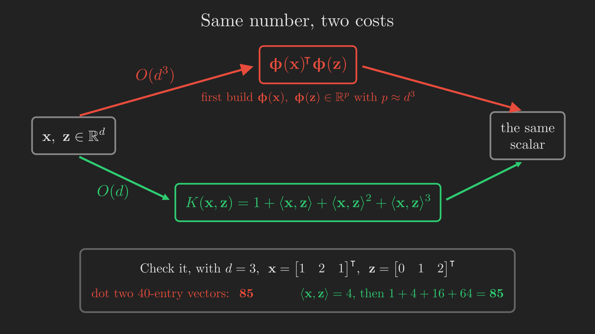
The explicit route builds \(\boldsymbol{\upphi}(\vb{x})\) and \(\boldsymbol{\upphi}(\vb{z})\), each with \(1 + 3 + 3^2 + 3^3 = 40\) entries, and dots them together: forty multiplications and thirty-nine additions, and the answer is \(85\). The kernel route computes \(\left\langle \vb{x}, \vb{z} \right\rangle = 1 \cdot 0 + 2 \cdot 1 + 1 \cdot 2 = 4\) and then
\[ 1 + 4 + 4^{2} + 4^{3} = 1 + 4 + 16 + 64 = 85. \]
The same \(85\), from three multiplications and a handful of additions. Nothing was approximated and nothing was thrown away; the two calculations are algebraically identical, and only one of them is expensive. Figure 6 puts both routes side by side.
This cheap-to-evaluate stand-in for the feature inner product is important enough to get a name and a symbol. We define the kernel corresponding to a feature map \(\boldsymbol{\upphi}\) as the function \(K : \mathcal{X} \times \mathcal{X} \to \mathbb{R}\) given by
\[ K(\vb{x}, \vb{z}) \triangleq \left\langle \boldsymbol{\upphi}(\vb{x}), \boldsymbol{\upphi}(\vb{z}) \right\rangle, \tag{11}\]
where \(\mathcal{X}\) is the space the attributes live in (for our running example, \(\mathcal{X} = \mathbb{R}^d\)). For the degree-\(\leq 3\) map, Equation 10 tells us \(K(\vb{x}, \vb{z}) = 1 + \left\langle \vb{x}, \vb{z} \right\rangle + \left\langle \vb{x}, \vb{z} \right\rangle^{2} + \left\langle \vb{x}, \vb{z} \right\rangle^{3}\).
The Kernelized Algorithm
We now have all the pieces. Let us assemble them into a clean procedure. Define the \(n \times n\) kernel matrix (also called the Gram matrix) \(\vb{K}\) by \(K_{ij} = K(\vb{x}_i, \vb{x}_j)\). Precompute it once. Then iterate the coefficient update, which per coordinate reads
\[ \forall\, i \in \{1, \ldots, n\}, \quad \beta_i := \beta_i + \alpha \left( y_i - \sum_{j=1}^{n} \beta_j K_{ij} \right), \tag{12}\]
and which, written in one line for the whole vector \(\boldsymbol{\upbeta}\) at once, is
\[ \boldsymbol{\upbeta} := \boldsymbol{\upbeta} + \alpha \left( \vb{y} - \vb{K} \boldsymbol{\upbeta} \right). \tag{13}\]
Here \(\vb{y} = \begin{bmatrix} y_1 & \cdots & y_n \end{bmatrix}^{\intercal}\) stacks the targets. One implementation detail hides in the difference between these two lines, and it is worth spelling out because it is easy to get wrong: all \(n\) updates in Equation 12 use the old \(\boldsymbol{\upbeta}\) on the right-hand side. If you loop over \(i\) and overwrite \(\beta_i\) in place, later coordinates will see already-updated earlier ones, and you will be running a subtly different algorithm. The vector form Equation 13 enforces the right thing automatically, which is one more reason to prefer it. Alg. 1 lays out the full method.
Algorithm 1
\begin{algorithm}
\caption{Kernelized LMS via batch gradient descent}
\begin{algorithmic}
\INPUT Examples $\vb{x}_1, \ldots, \vb{x}_n$ with targets $y_1, \ldots, y_n$; kernel $K$; learning rate $\alpha$; iterations $T$
\OUTPUT Coefficient vector $\boldsymbol{\upbeta} \in \mathbb{R}^n$
\STATE Precompute the kernel matrix $K_{ij} \leftarrow K(\vb{x}_i, \vb{x}_j)$ for all $i, j \in \{1, \ldots, n\}$
\STATE $\boldsymbol{\upbeta} \leftarrow \vb{0}$
\FOR{$t = 1$ \TO $T$}
    \STATE $\boldsymbol{\upbeta} \leftarrow \boldsymbol{\upbeta} + \alpha \left( \vb{y} - \vb{K} \boldsymbol{\upbeta} \right)$
\ENDFOR
\RETURN $\boldsymbol{\upbeta}$
\end{algorithmic}
\end{algorithm}
Each iteration of alg. 1 is a single matrix-vector product, \(O(n^2)\) work, with no reference to \(p\) anywhere. Building the kernel matrix up front costs \(n^2\) kernel evaluations, and each of those is \(O(d)\) thanks to the shortcut, so \(O(n^2 d)\) once, followed by \(O(n^2)\) per iteration. The dreaded \(d^3\) never appears.
It is worth being precise about what just happened, because it is easy to over-read. The feature space did not go away. Our model is still \(h(\vb{x}) = \boldsymbol{\uptheta}^{\intercal}\boldsymbol{\upphi}(\vb{x})\) with \(\boldsymbol{\uptheta}\) living in \(\mathbb{R}^p\), and \(p\) is still about \(d^3\). What vanished is our need to ever touch \(\boldsymbol{\uptheta}\) or \(\boldsymbol{\upphi}\) on a computer. The mathematics still happens in the billion-dimensional space; only the arithmetic escaped it.
What about prediction? Once training gives us \(\boldsymbol{\upbeta}\), the prediction on a fresh test point \(\vb{x}_{\text{test}}\) is
\[ \begin{align*} h_{\boldsymbol{\uptheta}}(\vb{x}_{\text{test}}) &= \boldsymbol{\uptheta}^{\intercal} \boldsymbol{\upphi}(\vb{x}_{\text{test}})\\ &= \sum_{i=1}^{n} \beta_i \, \boldsymbol{\upphi}(\vb{x}_i)^{\intercal} \boldsymbol{\upphi}(\vb{x}_{\text{test}})\\ \therefore h_{\boldsymbol{\uptheta}}(\vb{x}_{\text{test}}) &= \sum_{i=1}^{n} \beta_i \, K(\vb{x}_i, \vb{x}_{\text{test}}), \end{align*} \tag{14}\]
again expressed purely through the kernel. Take a moment to appreciate what Equation 13 and Equation 14 have in common:
ImportantThe one observation that makes it all work
Neither training (Equation 13) nor prediction (Equation 14) contains \(\boldsymbol{\upphi}(\vb{x})\) anywhere. The feature map has completely vanished. Every place it would have appeared, it appears only as a kernel value \(K(\cdot, \cdot)\), a single number we know how to compute cheaply. This is why we can afford feature spaces we could never even write down.
There is, however, no free lunch, and it is only fair to name the price. In ordinary linear regression, once we learned \(\boldsymbol{\uptheta}\) we could throw the training set away; a new prediction needed only the vector \(\boldsymbol{\uptheta}\). The kernelized version cannot do that. Look again at Equation 14: to predict on \(\vb{x}_{\text{test}}\) we must evaluate \(K(\vb{x}_i, \vb{x}_{\text{test}})\) against every training point \(\vb{x}_i\). So we are forced to carry the entire training set with us to test time. Figure 7 makes the arithmetic of a single prediction visible.
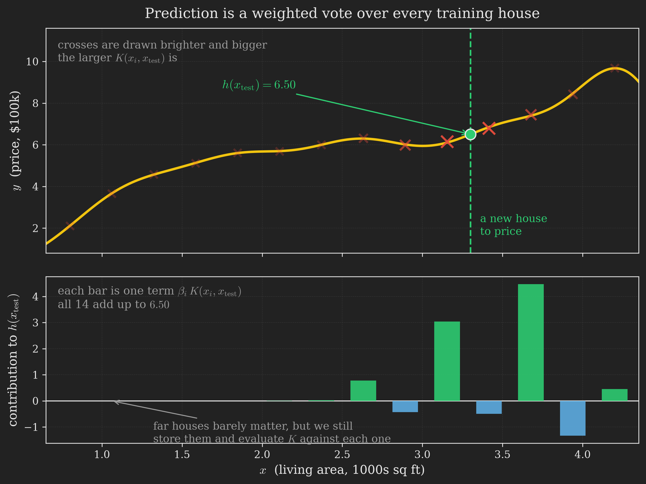
This is the characteristic trade of kernel methods. We gave up the compact parameter vector \(\boldsymbol{\uptheta}\), and in exchange we must remember the data. The cost shows up twice: the kernel matrix itself takes \(O(n^2)\) memory to store during training, and the whole training set has to be kept around afterwards for prediction. For small and medium datasets this is a fine bargain. Once \(n\) reaches the hundreds of thousands, an \(n \times n\) matrix stops fitting anywhere, which is one reason methods like deep neural networks, whose cost does not grow with the number of stored examples, tend to take over at large scale. (There is a partial escape: some kernel methods, notably the support vector machine we turn to next, learn a \(\boldsymbol{\upbeta}\) that is mostly zeros, so only a handful of examples, the “support vectors,” need to be kept. In Figure 7 that would mean most of those bars becoming exactly zero, and the houses under them getting thrown away for good.)
A quick recap before we change perspective
Let us pause at the clearing and look at the map. Figure 8 marks how far we have come.
flowchart TD
    A["Feature maps: x becomes ϕ(x)"] --> B["Plug into gradient descent"]
    B --> C["Wall: ϕ(x) is about d³"]
    C --> D["θ is a combo of the data"]
    D --> E["Rewrite with kernel K(x, z)"]
    E --> F["Done: ϕ has vanished"]
    F --> G["Next: choose K directly, without ϕ"]

    style F fill:#1e8449,color:#fff
    style G fill:#2471a3,color:#fff
So far we started from a feature map \(\boldsymbol{\upphi}\) and derived its kernel. But the algorithm we ended up with, alg. 1, never uses \(\boldsymbol{\upphi}\) at all; it only ever calls \(K\). That raises a delicious possibility: what if we forget feature maps entirely and just choose a kernel directly? That inversion is the subject of the rest of the post.
Kernels as Similarity
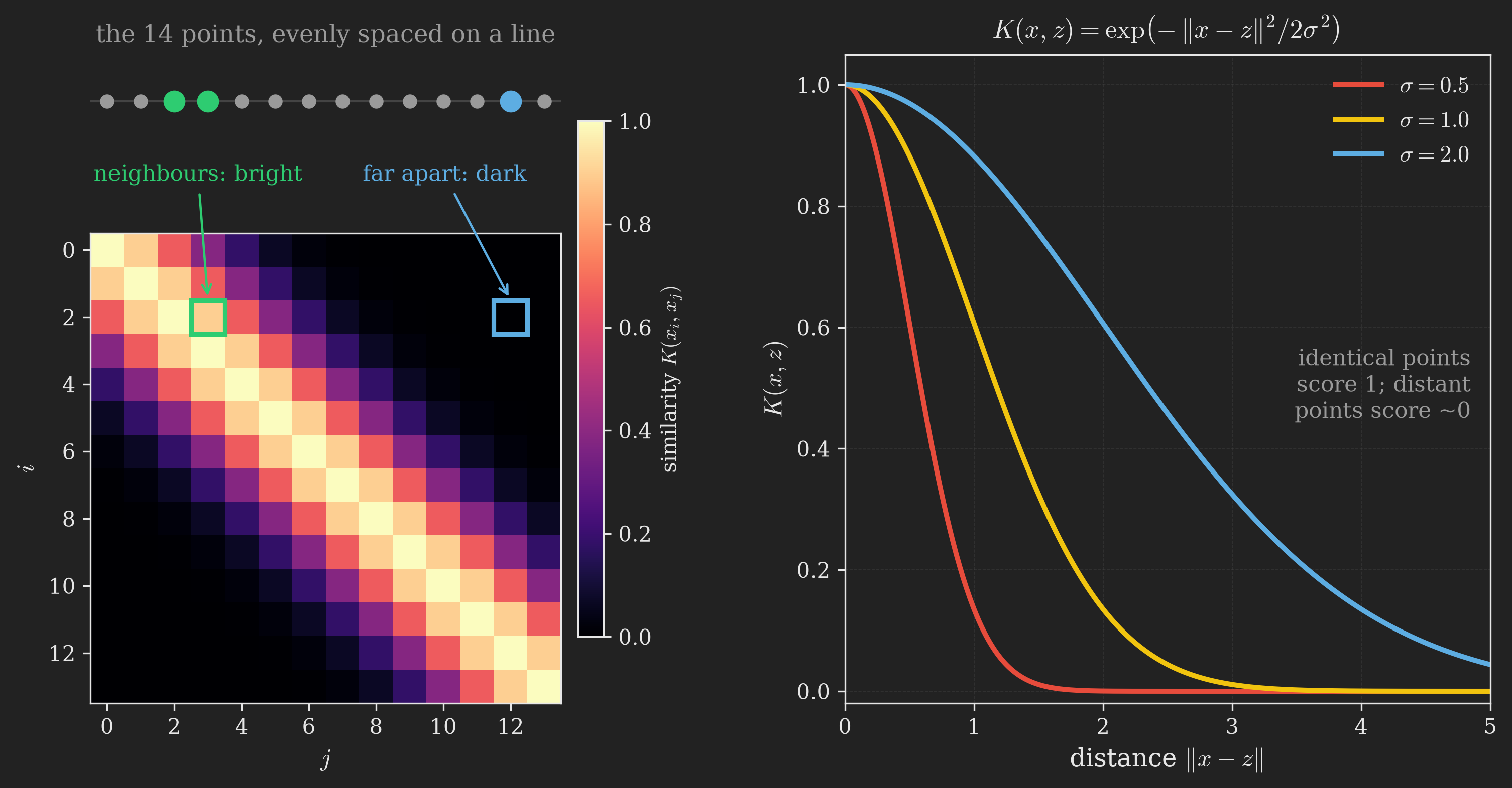
If we are going to pick kernels straight out of the air, it helps to have some intuition for what a kernel means. Here is a useful (if imperfect) way to think about it. Since \(K(\vb{x}, \vb{z}) = \left\langle \boldsymbol{\upphi}(\vb{x}), \boldsymbol{\upphi}(\vb{z}) \right\rangle\) is an inner product, and inner products are large for vectors pointing the same way and small (or negative) for vectors pointing apart, we can read \(K(\vb{x}, \vb{z})\) as a measure of how similar \(\vb{x}\) and \(\vb{z}\) are. Similar inputs, large kernel value; dissimilar inputs, small kernel value.
This flips the design process into something intuitive. Rather than asking “what features should I engineer?”, we ask “what does it mean for two of my inputs to be similar?”, and encode that answer as a kernel. A famous and enormously useful choice is the Gaussian kernel (also called the radial basis function or squared-exponential kernel):
\[ K(\vb{x}, \vb{z}) = \exp\left( -\frac{ \norm\big{\vb{x} - \vb{z}}^{2}}{2 \sigma^{2}} \right). \tag{15}\]
When \(\vb{x}\) and \(\vb{z}\) are close, \(\norm\big{\vb{x} - \vb{z}} \approx 0\) and \(K \approx 1\): maximal similarity. When they are far apart, the exponent is a large negative number and \(K \approx 0\): negligible similarity. The bandwidth \(\sigma\) sets how quickly “similar” fades into “unrelated.” Figure 9 shows both the resulting kernel matrix and the decay.
WarningHandle this intuition with care
The “kernel = similarity” picture is a helpful mental model, not a theorem. There are similarity-looking functions that are not valid kernels, and valid kernels whose values can be negative and so do not behave like a naive similarity score. Treat similarity as the inspiration for choosing a kernel, then verify validity with the test we develop below.
There is one near-collision worth naming explicitly. If you have met locally weighted regression, you have already seen the expression \(w_i = \exp\left( -\left(x_i - x\right)^2 / \left(2\tau^2\right) \right)\), which is character for character the Gaussian kernel of Equation 15. The formula is the same; the job is not. In locally weighted regression it is a weight, telling a plain linear fit how much to care about each training point near the query. Here it is an inner product in a feature space, telling us the geometry of the space our model lives in. Same bell curve, two entirely different roles, so resist the urge to conflate them.
The two ideas do rhyme in one uncomfortable way, though, and it is the reason both appear in this series: neither one lets you throw the training data away. Locally weighted regression refits around each query point; kernel methods evaluate \(K\) against every stored example. Flexibility bought with memory, twice over.
Two things about the Gaussian kernel are worth flagging now and will land fully in the next sections. It is trivially cheap to evaluate, one distance computation and one exponential, and yet, if you tried to write down the feature map \(\boldsymbol{\upphi}\) it secretly corresponds to, you would find it has infinitely many dimensions. We are computing inner products in an infinite-dimensional space in constant time. That is the whole promise of kernels, delivered.
The Payoff: Our Fourteen Houses, Revisited
We have been promising for a long time now. Let us collect.
Remember the fourteen houses from Figure 1, the ones whose S-shaped price curve defeated a straight line. We can now hand them to alg. 1 with a Gaussian kernel and see what comes out. Nothing else changes: same gradient descent, same targets, and at no point does anything in the computer hold a feature vector. Figure 10 shows the result at three bandwidths.
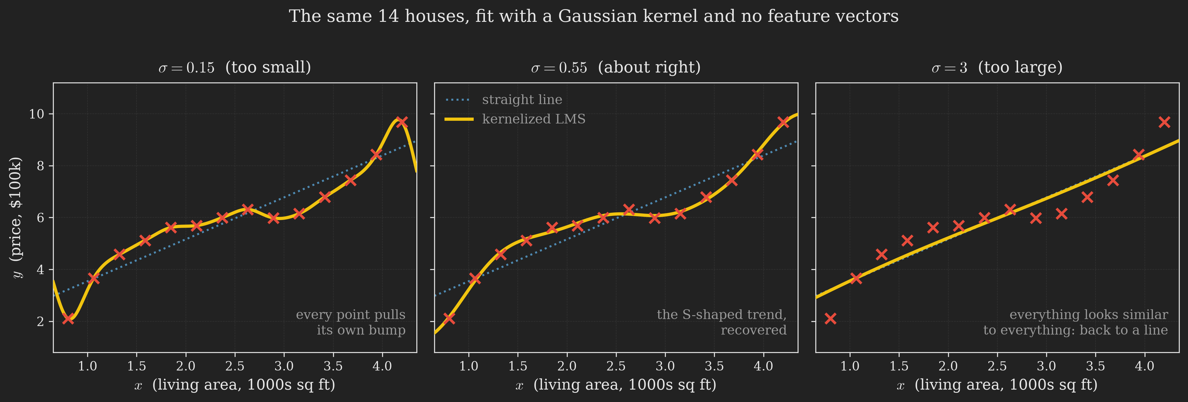
Look at what the middle panel cost us. We never decided “use a cubic.” We never wrote down \(\begin{bmatrix} 1 & x & x^2 & x^3 \end{bmatrix}^{\intercal}\). We picked a notion of similarity, turned the crank, and a curve came out. And the feature space that curve implicitly lives in is not four-dimensional or even a billion-dimensional; as the next sections will show, for the Gaussian kernel it is infinite-dimensional.
The right-hand panel is worth a second look too, because it is the cleanest possible statement of what \(\sigma\) does. Making the bandwidth huge means declaring that all our houses are roughly equally similar to one another, and a model that cannot tell its training points apart has nothing to work with but the overall trend. Flexibility, in kernel methods, is exactly a claim about which inputs count as alike.
(A small honest footnote on the figure: the kernel actually used is \(K(\vb{x}, \vb{z}) = 1 + \exp\left( -\norm\big{\vb{x} - \vb{z}}^{2} / \left(2\sigma^2\right) \right)\). The extra constant is what gives the model an intercept, and adding \(1\) to a kernel leaves it a kernel, as we are about to prove in general.)
So the machinery works. That success, though, was built on a kernel we pulled out of thin air, and it raises two questions we have so far dodged: what other kernels are there, and what exactly is the feature space each of them stands in for? The next section answers the first by collecting the standard catalogue, and the one after that answers the second properly.
A Gallery of Kernels
Let us collect a few concrete kernels and, for each, connect the compact formula back to an explicit feature map so the correspondence in Equation 11 feels real rather than magical.
The Quadratic Kernel
Take \(\vb{x}, \vb{z} \in \mathbb{R}^d\) and consider
\[ K(\vb{x}, \vb{z}) = \left( \vb{x}^{\intercal} \vb{z} \right)^{2}. \tag{16}\]
Expanding the square,
\[ \begin{align*} K(\vb{x}, \vb{z}) &= \left( \sum_{j=1}^{d} x_j z_j \right) \left( \sum_{k=1}^{d} x_k z_k \right)\\[0.5em] &= \sum_{j,k=1}^{d} (x_j x_k)(z_j z_k), \end{align*} \]
which is exactly \(\left\langle \boldsymbol{\upphi}(\vb{x}), \boldsymbol{\upphi}(\vb{z}) \right\rangle\) for the feature map that lists every product \(x_j x_k\). Written out for \(d = 3\),
\[ \boldsymbol{\upphi}(\vb{x}) = \begin{bmatrix} x_1 x_1\\ x_1 x_2\\ x_1 x_3\\ x_2 x_1\\ x_2 x_2\\ x_2 x_3\\ x_3 x_1\\ x_3 x_2\\ x_3 x_3 \end{bmatrix}. \]
Building this \(\boldsymbol{\upphi}(\vb{x})\) takes \(O(d^2)\) work, but evaluating \(K\) through Equation 16 takes only \(O(d)\): compute \(\vb{x}^{\intercal}\vb{z}\), then square. The shortcut again.
The Inhomogeneous Quadratic Kernel
A close relative adds a constant before squaring:
\[ \begin{align*} K(\vb{x}, \vb{z}) &= \left( \vb{x}^{\intercal} \vb{z} + c \right)^{2}\\[0.5em] &= \sum_{j,k=1}^{d} (x_j x_k)(z_j z_k) + \sum_{j=1}^{d} \left( \sqrt{2c}\, x_j \right)\left( \sqrt{2c}\, z_j \right) + c^{2}. \end{align*} \]
Matching the three groups of terms, its feature map (again shown for \(d = 3\)) keeps the same second-order products \(x_j x_k\) and adds the first-order terms \(\sqrt{2c}\, x_j\) and a constant \(c\):
\[ \boldsymbol{\upphi}(\vb{x}) = \begin{bmatrix} x_1 x_1\\ x_1 x_2\\ x_1 x_3\\ x_2 x_1\\ x_2 x_2\\ x_2 x_3\\ x_3 x_1\\ x_3 x_2\\ x_3 x_3\\ \sqrt{2c}\, x_1\\ \sqrt{2c}\, x_2\\ \sqrt{2c}\, x_3\\ c \end{bmatrix}. \]
The parameter \(c \geq 0\) tunes how much weight the model puts on the first-order (linear) terms relative to the second-order (interaction) terms.
The General Polynomial Kernel
Pushing the pattern, the kernel
\[ K(\vb{x}, \vb{z}) = \left( \vb{x}^{\intercal} \vb{z} + c \right)^{k} \]
corresponds to a feature space of all monomials up to degree \(k\), which has \(\binom{d + k}{k}\) dimensions, on the order of \(d^k\). And still, computing \(K\) costs only \(O(d)\). We never build the \(d^k\)-dimensional vector.
Table 1 gathers these, plus the linear and Gaussian kernels, in one place.
| Kernel | \(K(\vb{x}, \vb{z})\) | Feature-space dimension | Cost to evaluate |
|---|---|---|---|
| Linear | \(\vb{x}^{\intercal}\vb{z}\) | \(d\) | \(O(d)\) |
| Polynomial (degree \(k\)) | \(\left(\vb{x}^{\intercal}\vb{z} + c\right)^{k}\) | \(\binom{d+k}{k} \sim d^{k}\) | \(O(d)\) |
| Gaussian (RBF) | \(\exp\left( -\dfrac{ \norm\big{\vb{x} - \vb{z}}^{2}}{2 \sigma^{2}} \right)\) | \(\infty\) | \(O(d)\) |
Where we stand
Time for another look at the trail map. Figure 11 marks the shift that just happened and the question it leaves open.
flowchart TD
    A["Kernelized algorithm: only K appears"] --> B["Read K as a similarity score"]
    B --> C["Choose K directly: Gaussian, polynomial"]
    C --> D["It works: our 14 houses, fit"]
    D --> E["But which functions are legal kernels?"]
    E --> F["Mercer's theorem answers it"]

    style D fill:#1e8449,color:#fff
    style E fill:#c0392b,color:#fff
    style F fill:#2471a3,color:#fff
The red box is the loose thread. We have been picking kernels out of the air with nothing but intuition to justify it, and intuition, as the warning above admitted, is not a proof. Time to tighten that.
Which Functions Are Valid Kernels? Mercer’s Theorem
We have been cavalier. We said “just choose a kernel,” but not every function \(K(\vb{x}, \vb{z})\) you scribble down is a legal kernel. To be legal, it must equal \(\left\langle \boldsymbol{\upphi}(\vb{x}), \boldsymbol{\upphi}(\vb{z}) \right\rangle\) for some feature map \(\boldsymbol{\upphi}\); otherwise the whole derivation that justified alg. 1 collapses. So the crucial question is:
Given a function \(K(\cdot, \cdot)\), how can we tell whether some feature map \(\boldsymbol{\upphi}\) exists with \(K(\vb{x}, \vb{z}) = \boldsymbol{\upphi}(\vb{x})^{\intercal}\boldsymbol{\upphi}(\vb{z})\), without having to construct \(\boldsymbol{\upphi}\) by hand?
The beauty of the answer is that we never need to exhibit \(\boldsymbol{\upphi}\); we only need to know it exists. Let us first find properties every valid kernel must have, then learn that those properties are also enough.
Necessary Conditions
Suppose \(K\) is valid, so \(K(\vb{x}, \vb{z}) = \boldsymbol{\upphi}(\vb{x})^{\intercal}\boldsymbol{\upphi}(\vb{z})\). Pick any finite set of points \(\left\{ \vb{x}_1, \ldots, \vb{x}_n \right\}\) (not necessarily the training set, any points at all) and form the kernel matrix \(\vb{K}\) with \(K_{ij} = K(\vb{x}_i, \vb{x}_j)\). Two properties follow immediately.
Symmetry. Since an inner product does not care about the order of its arguments,
\[ \begin{align*} K_{ij} &= \boldsymbol{\upphi}(\vb{x}_i)^{\intercal}\boldsymbol{\upphi}(\vb{x}_j)\\ &= \boldsymbol{\upphi}(\vb{x}_j)^{\intercal}\boldsymbol{\upphi}(\vb{x}_i)\\ &= K_{ji}, \end{align*} \]
so \(\vb{K}\) is symmetric.
Positive semidefiniteness. Let \(\phi_k(\vb{x})\) denote the \(k\)-th coordinate of \(\boldsymbol{\upphi}(\vb{x})\), and let \(\vb{c} \in \mathbb{R}^n\) be an arbitrary vector we use to probe the matrix. (The CS229 notes call this vector \(\vb{z}\), but \(\vb{z}\) is already doing duty as an input point everywhere else in this post, so we rename it here.) Then
\[ \begin{align*} \vb{c}^{\intercal} \vb{K} \vb{c} &= \sum_{i} \sum_{j} c_i K_{ij} c_j\\ &= \sum_{i} \sum_{j} c_i \, \boldsymbol{\upphi}(\vb{x}_i)^{\intercal} \boldsymbol{\upphi}(\vb{x}_j) \, c_j \\ &= \sum_{i} \sum_{j} c_i \left( \sum_{k} \phi_k(\vb{x}_i)\, \phi_k(\vb{x}_j) \right) c_j\\ &= \sum_{k} \sum_{i} \sum_{j} \left( c_i \phi_k(\vb{x}_i) \right)\left( c_j \phi_k(\vb{x}_j) \right) \\ &= \sum_{k} \left( \sum_{i} c_i \, \phi_k(\vb{x}_i) \right)^{2} \;\geq\; 0. \end{align*} \]
The last equality uses the identity \(\sum_{i,j} a_i a_j = \left( \sum_i a_i \right)^2\) with \(a_i = c_i \phi_k(\vb{x}_i)\). Because \(\vb{c}\) was arbitrary and the result is always a sum of squares, \(\vb{K}\) is positive semidefinite.
So every valid kernel produces symmetric, positive semidefinite kernel matrices, on every finite set of points. The remarkable fact, due to Mercer, is that this necessary condition is also sufficient.
TipMercer’s theorem
Let \(K : \mathbb{R}^d \times \mathbb{R}^d \to \mathbb{R}\) be given. Then \(K\) is a valid (Mercer) kernel, meaning there exists a feature map \(\boldsymbol{\upphi}\) with \(K(\vb{x}, \vb{z}) = \boldsymbol{\upphi}(\vb{x})^{\intercal}\boldsymbol{\upphi}(\vb{z})\), if and only if for every finite collection \(\left\{ \vb{x}_1, \ldots, \vb{x}_n \right\}\) (with \(n < \infty\)), the corresponding kernel matrix \(\vb{K} \in \mathbb{R}^{n \times n}\) is symmetric and positive semidefinite.
This is a genuinely powerful tool, because it lets us certify a kernel without ever finding its feature map (Hastie et al., 2009; Schölkopf & Smola, 2002). We get three complementary ways to prove a candidate function \(K\) is a kernel:
- Construct a feature map:
- Exhibit an explicit \(\boldsymbol{\upphi}\) with \(K(\vb{x}, \vb{z}) = \boldsymbol{\upphi}(\vb{x})^{\intercal}\boldsymbol{\upphi}(\vb{z})\), as we did for the polynomial kernels above.
- Check symmetry and positive semidefiniteness:
- Verify the Mercer condition directly, which is often far easier than hunting for \(\boldsymbol{\upphi}\), especially for something like the Gaussian kernel whose feature map is infinite-dimensional.
- Verify the continuous version of the same condition:
- Show that \(\displaystyle \int\!\!\int f(\vb{x})\, K(\vb{x}, \vb{x}')\, f(\vb{x}')\, \dd{\vb{x}} \dd{\vb{x}'} \;\geq\; 0\) for every square-integrable function \(f\). This is the same statement as (2) with the finite sums replaced by integrals and the probe vector \(\vb{c}\) replaced by a probe function \(f\). It is usually the hardest of the three to check by hand, but it is the form in which Mercer’s theorem is often stated, so it is worth recognizing.
Picturing the theorem
Routes (2) and (3) look like different statements, and the picture that reconciles them is worth carrying around. Imagine the kernel \(K\) as one enormous matrix, with a row for every possible input \(\vb{x}\) and a column for every possible input \(\vb{z}\), its \((\vb{x}, \vb{z})\) entry being the number \(K(\vb{x}, \vb{z})\). Choosing \(n\) points is choosing \(n\) rows and the matching \(n\) columns, and the kernel matrix \(\vb{K}\) is exactly the little submatrix sitting where they cross. Figure 12 draws it.
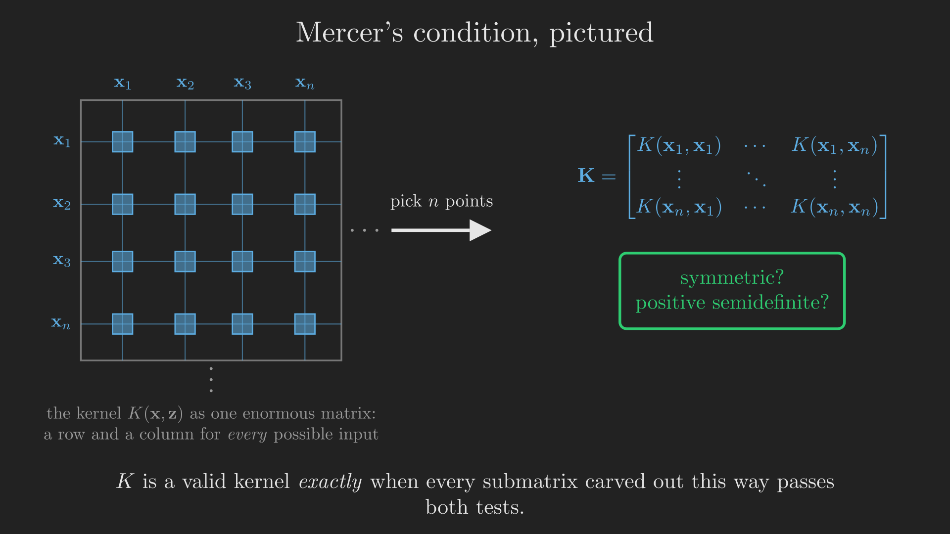
Route (3) is the assertion that the infinite object itself is positive semidefinite; route (2) is the assertion that every finite piece of it is. Mercer’s theorem says the two are equivalent, which is really just the familiar fact that any principal submatrix of a positive semidefinite matrix is itself positive semidefinite, promoted to the infinite-dimensional setting.
The test, run
Route (2) is not just theoretically convenient; it is something you can literally execute. Pick some points, build the matrix, ask a computer for its eigenvalues, and look for a negative one. Figure 13 does this for two functions that both look like perfectly reasonable similarity scores.
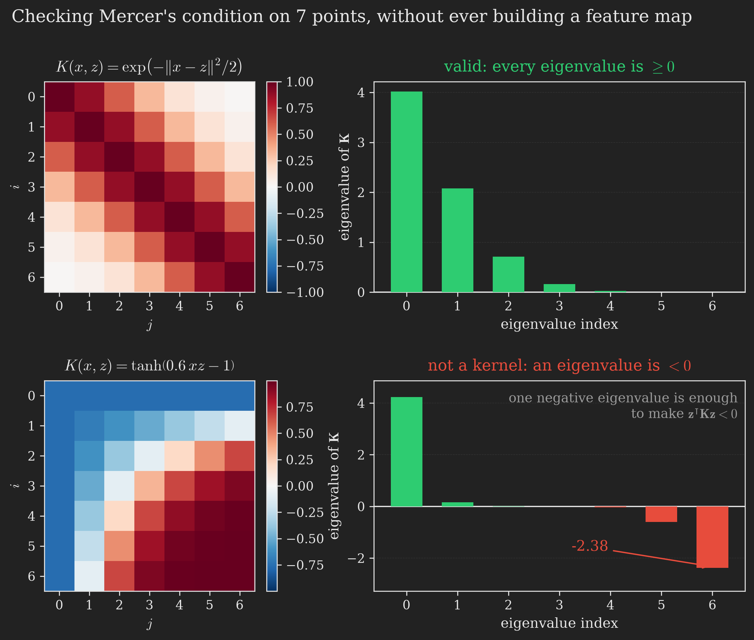
The bottom row deserves a moment. A single negative eigenvalue \(\lambda < 0\) with eigenvector \(\vb{c}\) gives \(\vb{c}^{\intercal}\vb{K}\vb{c} = \lambda \norm\big{\vb{c}}^{2} < 0\), which directly contradicts the chain of equalities we just proved must hold for any valid kernel. One counterexample on seven arbitrary points is enough to disqualify a function forever. This is also a fair warning about the “kernel = similarity” intuition: the sigmoid kernel is a perfectly sensible-looking similarity score, it is used in real software, and it is not a kernel.
Building New Kernels From Old Ones
There is a fourth route, and in practice it is the one people reach for most. Kernels are closed under a handful of operations, so once you have a few, you can manufacture endless others without going anywhere near a feature map or an eigenvalue.
Suppose \(K_1\) and \(K_2\) are valid kernels on \(\mathcal{X}\). Then all of the following are valid kernels too (Bishop, 2006; Schölkopf & Smola, 2002):
| Construction | New kernel | Why it works |
|---|---|---|
| Sum | \(K_1(\vb{x}, \vb{z}) + K_2(\vb{x}, \vb{z})\) | Stack the two feature maps into one longer vector |
| Positive scaling | \(a\, K_1(\vb{x}, \vb{z})\), for \(a > 0\) | Scale the feature map by \(\sqrt{a}\) |
| Constant | \(c\), for \(c \geq 0\) | The feature map is the single number \(\sqrt{c}\) |
| Product | \(K_1(\vb{x}, \vb{z})\, K_2(\vb{x}, \vb{z})\) | The feature map lists all products \(\phi^{(1)}_j(\vb{x}) \phi^{(2)}_k(\vb{x})\) |
| Rescaling by a function | \(f(\vb{x})\, K_1(\vb{x}, \vb{z})\, f(\vb{z})\), any \(f\) | Multiply the feature map through by \(f(\vb{x})\) |
| Limits | \(\lim_{m \to \infty} K_m(\vb{x}, \vb{z})\), if it exists | Positive semidefiniteness survives taking limits |
Two of these we have already used without comment. Back in Figure 10 the kernel was \(1 + \exp\left( -\norm\big{\vb{x} - \vb{z}}^{2} / \left(2\sigma^2\right) \right)\), which is legal by the “constant” and “sum” rules. And the polynomial kernel of Equation 10, \(1 + \left\langle \vb{x}, \vb{z} \right\rangle + \left\langle \vb{x}, \vb{z} \right\rangle^2 + \left\langle \vb{x}, \vb{z} \right\rangle^3\), is now a one-line proof: the linear kernel \(\left\langle \vb{x}, \vb{z} \right\rangle\) is a kernel, products of kernels are kernels (so its square and cube are), constants are kernels, and sums of kernels are kernels. We spent a page expanding monomials earlier to prove exactly that. The closure rules get it for free.
NoteCashing the cheque: the Gaussian kernel really is a kernel
We have twice promised that the Gaussian kernel corresponds to an infinite-dimensional feature map, and twice moved on without proving it. The closure rules let us settle it in a few lines.
Start by expanding the exponent:
\[ \norm\big{\vb{x} - \vb{z}}^{2} = \norm\big{\vb{x}}^{2} - 2 \left\langle \vb{x}, \vb{z} \right\rangle + \norm\big{\vb{z}}^{2}, \]
so that the Gaussian kernel factors as
\[ K(\vb{x}, \vb{z}) = \underbrace{\exp\left( -\frac{\norm\big{\vb{x}}^{2}}{2\sigma^{2}} \right)}_{f(\vb{x})} \cdot \underbrace{\exp\left( \frac{\left\langle \vb{x}, \vb{z} \right\rangle}{\sigma^{2}} \right)}_{\text{the interesting part}} \cdot \underbrace{\exp\left( -\frac{\norm\big{\vb{z}}^{2}}{2\sigma^{2}} \right)}_{f(\vb{z})}. \tag{17}\]
The outer two factors of Equation 17 are exactly the “rescaling by a function” row of Table 2, with \(f(\vb{x}) = \exp\left( -\norm\big{\vb{x}}^{2} / \left(2\sigma^2\right) \right)\). So the whole thing is a valid kernel as soon as the middle factor is. And the middle factor yields to the power series of the exponential:
\[ \exp\left( \frac{\left\langle \vb{x}, \vb{z} \right\rangle}{\sigma^{2}} \right) = \sum_{m=0}^{\infty} \frac{1}{m!\, \sigma^{2m}} \left\langle \vb{x}, \vb{z} \right\rangle^{m}. \]
Every term is a non-negative constant times a power of the linear kernel, so every term is a kernel by the product and scaling rules; the partial sums are kernels by the sum rule; and the limit is a kernel by the limit rule. The Gaussian kernel is therefore valid, and the argument also tells us why its feature space is infinite-dimensional: the series never terminates, so the implied feature map contains monomials of every degree, all the way up. A cubic feature map gives you degree three. The Gaussian gives you all of them at once, for one exponential.
That closes the last open question. We know what a kernel is, we know how to check whether a candidate function qualifies, we know how to build new ones out of old ones, and we have watched one fit real data. The only thing left is to see how far outside linear regression the idea travels, which turns out to be a very long way indeed.
Why This Matters: The Reach of the Kernel Trick
It would be a shame to leave the impression that kernels are a party trick for polynomial regression. They are a general lever, and it is worth seeing how far it reaches.
Recognizing handwritten digits. Consider classifying \(16 \times 16\)-pixel images of handwritten digits, so each input is a raw \(256\)-dimensional vector of pixel intensities. Feeding those pixels to a support vector machine with a plain polynomial kernel \(K(\vb{x}, \vb{z}) = \left( \vb{x}^{\intercal}\vb{z} \right)^k\) or a Gaussian kernel already achieves excellent accuracy (Schölkopf & Smola, 2002). What makes this striking is that the model is handed no prior knowledge about vision, not even which pixels are neighbors, and still learns to read digits. The kernel silently manufactures a rich feature space of pixel interactions that the linear machinery on top can exploit.
Comparing strings and proteins. Suppose the inputs are not vectors but strings, say sequences of amino acids that fold into proteins, of different lengths. Hand-engineering a fixed feature vector for such objects is painful. But define \(\boldsymbol{\upphi}(\vb{x})\) to count how many times each length-\(k\) substring occurs in \(\vb{x}\). For strings over the 26 letters, that is a \(26^k\)-dimensional vector, hopelessly large even for modest \(k\) (already \(26^4 \approx 460{,}000\)). Yet the corresponding kernel \(K(\vb{x}, \vb{z}) = \boldsymbol{\upphi}(\vb{x})^{\intercal}\boldsymbol{\upphi}(\vb{z})\) can be computed efficiently with dynamic-programming-style string-matching algorithms, so we work implicitly in that gigantic feature space while never building a single feature vector (Schölkopf & Smola, 2002).
Kernelize almost anything. The deepest point is a recipe. If you can write a learning algorithm so that inputs appear only through inner products \(\left\langle \vb{x}, \vb{z} \right\rangle\), then replacing every such inner product with a kernel \(K(\vb{x}, \vb{z})\) instantly upgrades the algorithm to work in the kernel’s high-dimensional feature space, at no extra asymptotic cost. This “kernel trick” is not specific to regression:
- Apply it to the perceptron and you get the kernel perceptron.
- Apply it to the generalized linear models from the exponential family and GLMs post, for instance logistic or Poisson regression, and you get their kernelized versions.
- Apply it to principal component analysis, which is built entirely out of inner products, and you get kernel PCA: principal directions in a feature space you never construct. That is an unsupervised algorithm, with no labels anywhere, which shows the trick has nothing to do with supervision (Schölkopf & Smola, 2002).
- It works for discriminative and generative models, and for supervised and unsupervised learning alike.
One more destination is worth naming because it takes the “kernel as similarity” reading completely seriously. In a Gaussian process, the kernel is not a computational shortcut hidden inside an algorithm; it is the model. You specify how similar any two inputs are, and that specification alone determines a distribution over functions. The similarity intuition we were careful to hedge earlier becomes, in that setting, the whole modelling language (Bishop, 2006).
The kernel idea is, in short, a general-purpose amplifier for any inner-product-based algorithm (Bishop, 2006).
Conclusion: What We Gained, and Where We Go Next
Let us close the loop we opened with a curve that a straight line could not fit.
That loop is, quite literally, closed. The fourteen houses of Figure 1 are the same fourteen houses of Figure 10, and the S-shaped trend that defeated the line in the first figure is tracked cleanly in the second. What sits between those two pictures is everything this post was about.
We started by noticing that a nonlinear fit is just a linear fit over cleverly chosen features, and we packaged that idea as a feature map \(\boldsymbol{\upphi}\). Plugging \(\boldsymbol{\upphi}\) into gradient descent was effortless, until the features exploded to \(d^3\) (or worse) dimensions and threatened to make everything a million times slower. Then came the three-step rescue:
- Started from \(\boldsymbol{\uptheta} = \vb{0}\), the parameter \(\boldsymbol{\uptheta}\) always stays a combination \(\sum_i \beta_i \boldsymbol{\upphi}(\vb{x}_i)\) of the data, so we can track \(n\) coefficients instead of \(p\) weights.
- Rewritten in terms of those coefficients, the algorithm touches the features only through inner products \(\left\langle \boldsymbol{\upphi}(\vb{x}_i), \boldsymbol{\upphi}(\vb{x}_j) \right\rangle\).
- Those inner products collapse into a cheap kernel \(K(\vb{x}, \vb{z})\), so the feature map vanishes from both training and prediction.
The real prize is a decoupling. We separated the question of what features to use from the question of how much it costs to compute. Once decoupled, we could reach for feature spaces of astronomical or even infinite dimension, and pay only \(O(d)\) per kernel evaluation. Mercer’s theorem then told us precisely which functions we are allowed to use as kernels: the symmetric, positive semidefinite ones. And the closure rules of Table 2 turned that licence into a construction kit, one that let us finally prove what we had been claiming all along, that the Gaussian kernel’s feature space really is infinite-dimensional.
The one cost we accepted along the way was memory: without a compact \(\boldsymbol{\uptheta}\), we must keep the training data around to make predictions, and the kernel matrix itself costs \(O(n^2)\) to store while we train. That very concern sets up the next chapter. In the next post we turn to the support vector machine, an algorithm that not only pairs beautifully with kernels but also, through its notion of a margin, learns a coefficient vector \(\boldsymbol{\upbeta}\) that is mostly zeros, so only a few “support vectors” need to be remembered. Kernels gave us the power to work in vast feature spaces; support vector machines will show us how to use that power to draw the best possible boundary.
References
Bishop, C. M. (2006). Pattern Recognition and Machine Learning. Springer.
Hastie, T., Tibshirani, R., Friedman, J., et al. (2009). The Elements of Statistical Learning: Data Mining, Inference, and Prediction. Springer series in statistics New-York.
Ng, A., & Ma, T. (2023). CS229 Lecture Notes. Stanford University; https://cs229.stanford.edu/main_notes.pdf.
Schölkopf, B., & Smola, A. J. (2002). Learning with Kernels: Support Vector Machines, Regularization, Optimization, and Beyond. MIT Press.
Stanford Online, Anand Avati. (2019). Stanford CS229: Machine Learning Course | Summer 2019. Stanford University; https://youtube.com/playlist?list=PLoROMvodv4rNH7qL6-efu_q2_bPuy0adh.