flowchart TD
    A["Which line separates the classes best?"] --> B["Confidence = distance from the boundary"]
    B --> C["Functional margin (gameable by rescaling)"]
    C --> D["Geometric margin (the true distance)"]
    D --> E["Maximize the margin: a convex QP"]
    E --> F["Lagrange duality + KKT conditions"]
    F --> G["Dual form: only inner products, sparse support vectors"]
    G --> H["Kernels plug in: nonlinear boundaries"]
    H --> I["Soft margin + hinge loss: handle outliers"]
    I --> J["SMO: solve the dual efficiently"]

    style E fill:#c0392b,color:#fff
    style G fill:#1e8449,color:#fff
    style H fill:#2471a3,color:#fff
Support Vector Machines
Machine Learning
Supervised Learning
Mathematics
A first-principles tour of support vector machines: from the intuition of a maximum-margin classifier, through functional and geometric margins, the optimal margin classifier, Lagrange duality and the KKT conditions, the dual form that exposes support vectors and inner products, kernels, the soft margin and hinge loss, and finally the SMO algorithm that solves it all.
Where We Left Off
In the kernel methods post, we discovered something almost magical: by writing a learning algorithm so that the data appears only through inner products, we could work in feature spaces of astronomical, even infinite, dimension while paying only a tiny cost per kernel evaluation. But that post ended on an honest note about a price we had to pay. Because the kernelized model keeps a coefficient \(\beta_i\) for every training example, we had to drag the entire training set along to make a prediction. And then we dropped a hint:
There is a partial escape: some kernel methods, notably the support vector machine, learn a \(\boldsymbol{\upbeta}\) that is mostly zeros, so only a handful of examples, the “support vectors,” need to be kept.
This post makes good on that hint. The support vector machine (SVM) is widely regarded as one of the best “off-the-shelf” supervised learning algorithms we have (Cortes & Vapnik, 1995). It pairs beautifully with kernels, and its guiding idea, the margin, does two things at once: it draws the best possible boundary between two classes, and it forces most of those \(\beta_i\) coefficients to zero. Only the few examples sitting right at the frontier survive. Those are the support vectors, and they give the algorithm its name.
This post is largely based on the CS229 lecture notes by Ng & Ma (2023) and the accompanying lecture (Stanford Online, Anand Avati, 2019). For intuition, I lean heavily on the wonderful video series on SVMs by Kharkar (2020). Along the way we will cite the original SVM paper (Cortes & Vapnik, 1995), John Platt’s SMO algorithm (Platt, 1998), the standard convex optimization reference (Boyd & Vandenberghe, 2004), and the usual textbooks (Bishop, 2006; Hastie et al., 2009; Schölkopf & Smola, 2002) for deeper treatments.
A concrete question: which line?
Let us anchor everything in a small, relatable problem. Suppose we want to predict whether a student gets into their top-choice medical school. For each student we record two numbers, a (standardized) GPA and a (standardized) MCAT score, and we plot them: green triangles are students who got in (we will label them \(y = +1\)), red crosses are students who did not (\(y = -1\)). Higher scores tend to mean admission, so the two groups separate rather cleanly, as in Figure 1.
Now I ask you to draw a straight line that separates the two classes. Here is the catch: there are infinitely many such lines. Figure 1 shows three of them, and all three perfectly separate the training data we happen to have.
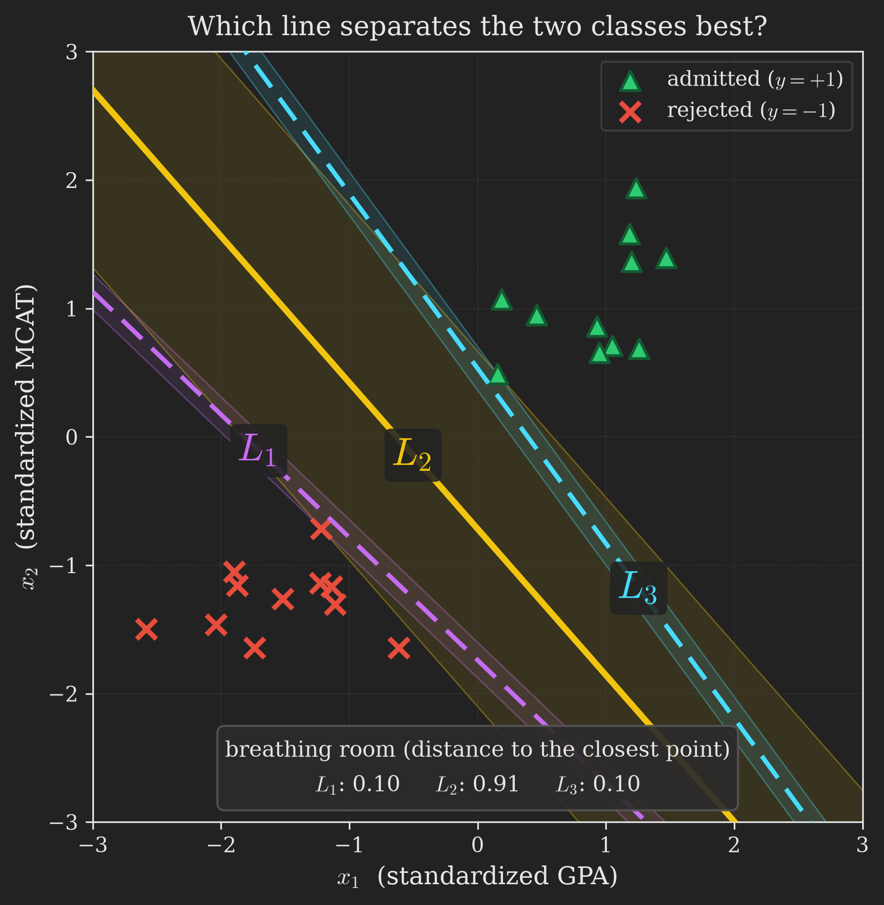
Which one is best? Almost everyone points at \(L_2\), and their instinct is exactly right. Line \(L_1\) skims right past the rejected students; a new rejected student who scored a touch higher than usual would fall on the wrong side of it. Line \(L_3\) has the same problem mirrored on the admitted side. Line \(L_2\) is the Goldilocks choice: it sits in the middle of the gap, as far from both clusters as it can be, so it has the most breathing room to absorb new, slightly unusual students (Kharkar, 2020).
The shaded corridors in Figure 1 make that comparison concrete rather than rhetorical. Each corridor is drawn as wide as it can be without swallowing a training point, so its half-width is precisely the distance from the line to the closest student. For \(L_1\) and \(L_3\) that distance is \(0.10\); for \(L_2\) it is \(0.91\). Eyeballing was right, and now we have a number attached to it. That number is the thing this entire post is about: name it, and then maximize it.
That single idea, prefer the boundary with the most breathing room, is the entire soul of the support vector machine. Everything else in this post is the machinery needed to make “the most breathing room” precise and then to compute it. The width of that breathing room has a name: the margin. An SVM is, in one phrase, a maximum-margin classifier.
The roadmap
Before we start building, here is the whole trail on one map. We begin with the fuzzy notion of “confidence,” sharpen it into two precise kinds of margin, turn “maximize the margin” into a clean optimization problem, take a necessary detour through Lagrange duality, and come out the other side with the dual form that reveals support vectors and lets kernels plug in. Then we make the method robust to messy real-world data and, finally, we solve it. Figure 2 sketches the journey.
The three highlighted boxes are the emotional beats of the story: turning intuition into a solvable problem (red), the dual form that changes everything (green), and the moment kernels enter (blue). Keep them in mind.
A note on the checkpoint diagrams you will meet along the way: in those, the colours mean something narrower and consistent. Green marks the step we have just finished, and blue marks the one we are about to take. Whenever you see a small version of this map, read it that way.
Confidence: How Sure Are We?
Let us start where Figure 1 left off, with the feeling that some predictions are safer than others. This intuition is easiest to see if we recall logistic regression. There, we modeled
\[ p(y = 1 \mid \vb{x}; \boldsymbol{\uptheta}) = h_{\boldsymbol{\uptheta}}(\vb{x}) = g\left(\boldsymbol{\uptheta}^{\intercal}\vb{x}\right), \]
with \(g\) the sigmoid, and we predicted “1” whenever \(\boldsymbol{\uptheta}^{\intercal}\vb{x} \geq 0\). But notice a finer point: the larger \(\boldsymbol{\uptheta}^{\intercal}\vb{x}\) is, the closer \(h_{\boldsymbol{\uptheta}}(\vb{x})\) gets to 1, and the more confident we feel that the label is really 1. So a prediction with \(\boldsymbol{\uptheta}^{\intercal}\vb{x} \gg 0\) is a confident “1,” and one with \(\boldsymbol{\uptheta}^{\intercal}\vb{x} \ll 0\) is a confident “0.”
Informally, then, we would love to find parameters so that \(\boldsymbol{\uptheta}^{\intercal}\vb{x}_i \gg 0\) whenever \(y_i = 1\) and \(\boldsymbol{\uptheta}^{\intercal}\vb{x}_i \ll 0\) whenever \(y_i = 0\). That would reflect confident and correct classifications on every training example. We will soon make this precise with functional margins.
There is a second, more geometric way to see the same thing. In Figure 3, three admitted students, A, B, and C, all sit on the correct (admitted) side of one particular boundary. But they are not equally convincing.
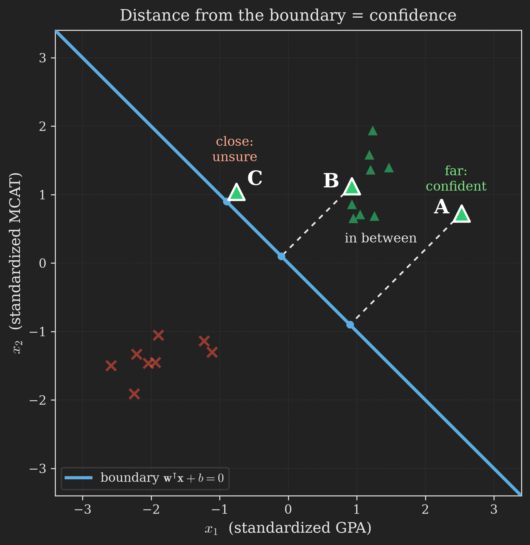
Point A is far from the boundary. If asked to bet on A, we would bet confidently that it is an admit. Point C sits right on top of the boundary; although it is on the admitted side today, the tiniest change to the line could put it on the other side. We are much more sure about A than about C, with B somewhere in between. The lesson: the farther a point is from the boundary, the more confident we can be about it. We will make this precise with geometric margins.
Both notions, functional and geometric, are about to become formulas. But first we need slightly cleaner notation.
A Cleaner Notation
For the rest of this post we adopt three notational changes that make the SVM story much smoother. None of them changes anything fundamental; they just tidy the algebra.
Labels are \(\pm 1\), not \(0/1\):
From now on, \(y \in \{-1, 1\}\) instead of \(\{0, 1\}\). The label \(+1\) is the positive class (admitted), \(-1\) is the negative class (rejected). This tiny change pays off constantly, because multiplying by \(y_i\) will let us fold “correct on a positive example” and “correct on a negative example” into a single expression.
Split off the intercept:
Rather than parameterizing our linear classifier with a single vector \(\boldsymbol{\uptheta}\) (and the trick of pinning \(x_0 = 1\)), we write the classifier with a separate weight vector \(\vb{w}\) and intercept \(b\):
\[ h_{\vb{w}, b}(\vb{x}) = g\left(\vb{w}^{\intercal}\vb{x} + b\right). \tag{1}\] Here \(\vb{w} \in \mathbb{R}^d\) plays the role of \(\left[\theta_1 \ \cdots \ \theta_d\right]^{\intercal}\), and \(b \in \mathbb{R}\) plays the role of the old \(\theta_0\). Keeping \(b\) explicit and separate will matter later (for instance, we will deliberately not penalize \(b\)).
Predict a hard label:
Our \(g\) is now a hard threshold, not a sigmoid:
\[ g(z) = \begin{cases} +1 & \text{if } z \geq 0,\\ -1 & \text{if } z < 0. \end{cases} \tag{2}\]
So the classifier in Equation 1 jumps straight to a \(\pm 1\) prediction, without ever estimating a probability in between (this is exactly what the perceptron did, in contrast to logistic regression).
With this notation in hand, we can finally define the two margins.
Functional and Geometric Margins
The functional margin
Given a single training example \(\left(\vb{x}_i, y_i\right)\), we define the functional margin of the parameters \((\vb{w}, b)\) with respect to that example as
\[ \hat{\gamma}_i = y_i\left(\vb{w}^{\intercal}\vb{x}_i + b\right). \tag{3}\]
Look at what this expression is doing, and why the \(\pm 1\) labels were a good idea. If \(y_i = +1\), then for Equation 3 to be large and positive we need \(\vb{w}^{\intercal}\vb{x}_i + b\) to be large and positive, which is exactly the “confident 1” we wanted. If \(y_i = -1\), then a large functional margin requires \(\vb{w}^{\intercal}\vb{x}_i + b\) to be large and negative, the “confident \(-1\).” In both cases:
- \(\hat{\gamma}_i > 0\) means the prediction is correct (the sign of \(\vb{w}^{\intercal}\vb{x}_i + b\) matches \(y_i\)). You can check this yourself by trying \(y_i = +1\) and \(y_i = -1\) separately.
- \(\hat{\gamma}_i \gg 0\) means the prediction is correct and confident.
So a large functional margin is precisely “confident and correct.” This is a promising thing to want to maximize. But there is a subtle flaw that we must confront before going further.
The scaling loophole. The classifier in Equation 1 depends only on the sign of \(\vb{w}^{\intercal}\vb{x} + b\), not its magnitude, because \(g\) is a hard threshold (Equation 2). So if we replace \((\vb{w}, b)\) with \((2\vb{w}, 2b)\), the actual decision boundary and every prediction stay exactly the same. And yet the functional margin doubles. Watch the two side by side:
Original parameters \((\vb{w}, b)\):
\[ \hat{\gamma}_i = y_i\left(\vb{w}^{\intercal}\vb{x}_i + b\right). \]
Scaled parameters \((2\vb{w}, 2b)\):
\[ y_i\left(2\vb{w}^{\intercal}\vb{x}_i + 2b\right) = 2\,\hat{\gamma}_i. \]
Same boundary, same classifier, but a functional margin twice as large. By scaling \(\vb{w}\) and \(b\) up without limit, we could make the functional margin as large as we like while changing nothing meaningful. This makes the raw functional margin a poor measure of confidence: it can be gamed (Stanford Online, Anand Avati, 2019). It cries out for a normalization, for instance insisting that \(\norm\big{\vb{w}} = 1\), so that scaling is no longer free. Hold that thought; the geometric margin will do exactly this.
Finally, we extend the definition from one example to a whole training set \(S = \left\{\left(\vb{x}_i, y_i\right); i = 1, \ldots, n\right\}\) by taking the worst (smallest) functional margin over all examples:
\[ \hat{\gamma} = \min_{i = 1, \ldots, n} \hat{\gamma}_i. \tag{4}\]
We take the minimum because a boundary is only as trustworthy as its shakiest example.
The geometric margin
The geometric margin fixes the scaling loophole by measuring the actual distance, in the units of the feature space, from a point to the decision boundary. Figure 4 sets up the geometry.
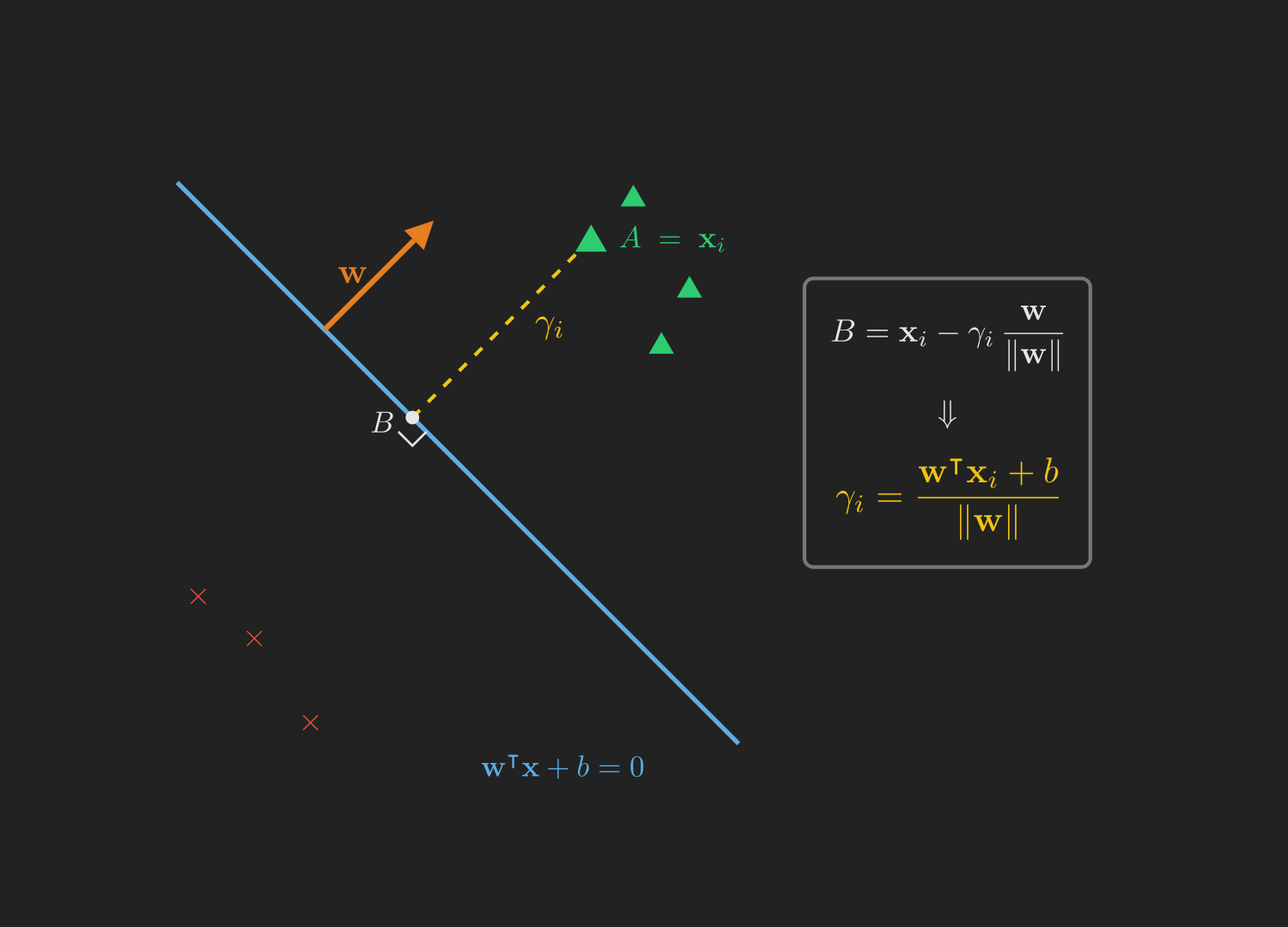
Two geometric facts drive the derivation. First, the vector \(\vb{w}\) is orthogonal to the separating hyperplane \(\vb{w}^{\intercal}\vb{x} + b = 0\). (Convince yourself: if \(\vb{x}\) and \(\vb{x}'\) both lie on the boundary, then \(\vb{w}^{\intercal}\vb{x} + b = 0\) and \(\vb{w}^{\intercal}\vb{x}' + b = 0\), so \(\vb{w}^{\intercal}(\vb{x} - \vb{x}') = 0\); the weight vector is perpendicular to every direction lying in the boundary.) Second, \(\vb{w}/\norm\big{\vb{w}}\) is the unit vector pointing in the direction of \(\vb{w}\).
Now consider the positive example at \(A = \vb{x}_i\), at distance \(\gamma_i\) from the boundary. To get from \(A\) to its foot \(B\) on the boundary, we walk a distance \(\gamma_i\) against the unit normal:
\[ B = \vb{x}_i - \gamma_i\,\frac{\vb{w}}{\norm\big{\vb{w}}}. \tag{5}\]
But \(B\) lies on the boundary, so it must satisfy \(\vb{w}^{\intercal}B + b = 0\). Substituting Equation 5,
\[ \vb{w}^{\intercal}\left(\vb{x}_i - \gamma_i\,\frac{\vb{w}}{\norm\big{\vb{w}}}\right) + b = 0. \tag{6}\]
Distributing \(\vb{w}^{\intercal}\) over the parentheses (and using \(\vb{w}^{\intercal}\vb{w} = \norm\big{\vb{w}}^2\), so that \(\vb{w}^{\intercal}\vb{w}/\norm\big{\vb{w}} = \norm\big{\vb{w}}\)), we solve Equation 6 for \(\gamma_i\):
\[ \begin{align*} \vb{w}^{\intercal}\left(\vb{x}_i - \gamma_i\,\frac{\vb{w}}{\norm\big{\vb{w}}}\right) + b &= 0\\ \implies \vb{w}^{\intercal}\vb{x}_i - \gamma_i\,\frac{\vb{w}^{\intercal}\vb{w}}{\norm\big{\vb{w}}} + b &= 0\\ \implies \vb{w}^{\intercal}\vb{x}_i - \gamma_i\,\norm\big{\vb{w}} + b &= 0\\ \implies \gamma_i &= \frac{\vb{w}^{\intercal}\vb{x}_i + b}{\norm\big{\vb{w}}}\\[0.3em] &= \left(\frac{\vb{w}}{\norm\big{\vb{w}}}\right)^{\intercal}\vb{x}_i + \frac{b}{\norm\big{\vb{w}}}. \end{align*} \tag{7}\]
This was worked out for a positive example, where being on the positive side is good. To handle both classes at once (there is the \(\pm 1\) trick paying off again), we multiply by \(y_i\) and define the geometric margin of \((\vb{w}, b)\) with respect to \(\left(\vb{x}_i, y_i\right)\) as
\[ \gamma_i = y_i\left(\left(\frac{\vb{w}}{\norm\big{\vb{w}}}\right)^{\intercal}\vb{x}_i + \frac{b}{\norm\big{\vb{w}}}\right). \tag{8}\]
Compare Equation 3 and Equation 8 side by side; the relationship is the whole point:
Functional margin:
\[ \hat{\gamma}_i = y_i\left(\vb{w}^{\intercal}\vb{x}_i + b\right). \]
Geometric margin:
\[ \begin{align*} \gamma_i &= y_i\left(\frac{\vb{w}^{\intercal}\vb{x}_i + b}{\norm\big{\vb{w}}}\right)\\[0.5em] \therefore \gamma_i &= \frac{\hat{\gamma}_i}{\norm\big{\vb{w}}}. \end{align*} \tag{9}\]
Two consequences follow immediately from Equation 9, and both matter later.
If \(\norm\big{\vb{w}} = 1\), the two margins are equal:
So the geometric margin is just the functional margin, normalized. This gives us a bridge between the two notions.
The geometric margin is immune to the scaling loophole:
Replace \((\vb{w}, b)\) with \((2\vb{w}, 2b)\): the numerator doubles, but so does \(\norm\big{\vb{w}}\) in the denominator, and \(\gamma_i\) is unchanged. It measures a genuine distance, so of course rescaling the parameters cannot move it.
That invariance is powerful in a way that is easy to miss. Because the geometric margin does not care how we scale \((\vb{w}, b)\), we are free to impose any one scaling constraint we like without changing a single geometric margin. We could demand \(\norm\big{\vb{w}} = 1\), or \(\left|w_1\right| = 5\), or \(\hat{\gamma} = 1\); each is just a choice of units. We will cash in this freedom very soon to turn an ugly optimization into a beautiful one.
As before, the geometric margin of \((\vb{w}, b)\) over the whole training set is the smallest one:
\[ \gamma = \min_{i = 1, \ldots, n} \gamma_i. \tag{10}\]
A first checkpoint
We have come a good distance already, so let us glance at the map. Figure 5 shows where we stand.
flowchart TD
    B["Confidence = distance from the boundary"] --> C["Functional margin (gameable)"]
    C --> D["Geometric margin (the true distance)"]
    D --> E["Next: maximize the geometric margin"]

    style D fill:#1e8449,color:#fff
    style E fill:#2471a3,color:#fff
We have a precise, scale-proof notion of how much breathing room a boundary has: the geometric margin \(\gamma\). The natural next move is obvious. Find the boundary that makes \(\gamma\) as large as possible.
The Optimal Margin Classifier
For now, assume our data is linearly separable: there really is some straight boundary with all positives on one side and all negatives on the other. (We will drop this assumption later, once we understand the clean case.) We want the boundary with the largest geometric margin \(\gamma\), because that is the most confident, most robust fit. We can write this as an optimization problem directly:
\[ \begin{aligned} \max_{\gamma, \vb{w}, b} \quad & \gamma \\ \text{s.t.} \quad & y_i\left(\vb{w}^{\intercal}\vb{x}_i + b\right) \geq \gamma, \quad i = 1, \ldots, n, \\ & \norm\big{\vb{w}} = 1. \end{aligned} \tag{11}\]
In words: maximize the margin \(\gamma\), subject to every example having (functional) margin at least \(\gamma\), and with \(\norm\big{\vb{w}} = 1\) so that functional and geometric margins coincide (making those constraints genuinely about geometric margin). If we could solve Equation 11, we would be done. Unfortunately, the constraint \(\norm\big{\vb{w}} = 1\) is nasty: it is non-convex (it pins \(\vb{w}\) to the surface of a sphere), and no standard optimizer will touch it. So we transform the problem into a friendlier shape.
Step 1: Get rid of the \(\norm\big{\vb{w}} = 1\) constraint
Recall from Equation 9 that \(\gamma = \hat{\gamma}/\norm\big{\vb{w}}\). So instead of constraining the geometric margin directly, we can maximize \(\hat{\gamma}/\norm\big{\vb{w}}\) subject to functional-margin constraints. Thus, Equation 11 becomes
\[ \begin{aligned} \max_{\hat{\gamma}, \vb{w}, b} \quad & \frac{\hat{\gamma}}{\norm\big{\vb{w}}} \\ \text{s.t.} \quad & y_i\left(\vb{w}^{\intercal}\vb{x}_i + b\right) \geq \hat{\gamma}, \quad i = 1, \ldots, n. \end{aligned} \tag{12}\]
We have traded the ugly constraint for an ugly (non-convex) objective \(\hat{\gamma}/\norm\big{\vb{w}}\). Not yet solvable, but we are close.
Step 2: Spend our scaling freedom
Here is where the invariance from the last section earns its keep. Since we may impose any one scaling constraint without changing the geometric margins, let us choose the convenient one
\[ \hat{\gamma} = 1. \tag{13}\]
That is, we rescale \((\vb{w}, b)\) so that the worst functional margin is exactly 1. With \(\hat{\gamma} = 1\), maximizing \(\hat{\gamma}/\norm\big{\vb{w}} = 1/\norm\big{\vb{w}}\) is the same as minimizing \(\norm\big{\vb{w}}\), which is the same as minimizing \(\tfrac{1}{2}\norm\big{\vb{w}}^2\) (the square and the \(\tfrac{1}{2}\) are just conveniences for the calculus later). We arrive at the clean problem
\[ \begin{aligned} \min_{\vb{w}, b} \quad & \frac{1}{2}\norm\big{\vb{w}}^2 \\ \text{s.t.} \quad & y_i\left(\vb{w}^{\intercal}\vb{x}_i + b\right) \geq 1, \quad i = 1, \ldots, n. \end{aligned} \tag{14}\]
This is the optimal margin classifier, and it is a thing of beauty: a convex quadratic objective with only linear constraints. This kind of problem, a quadratic program (QP), can be handed to standard commercial solvers and solved reliably.1 Its solution is the maximum-margin boundary.
A Geometric Sanity Check
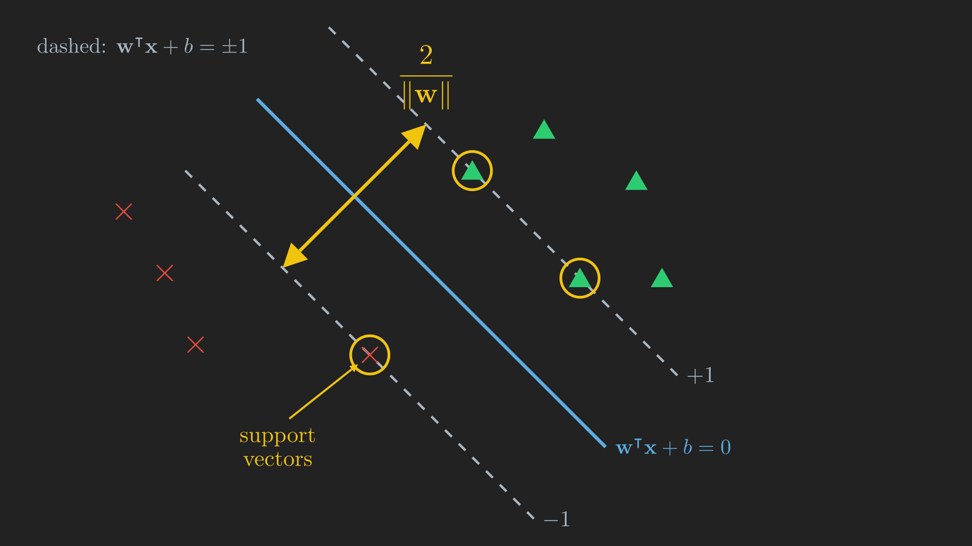
It is worth seeing “maximize the margin equals minimize \(\norm\big{\vb{w}}\)” from the pure geometry too, the way Kharkar (2020) tells it. With the scaling \(\hat{\gamma} = 1\), the closest positive examples land exactly on the line \(\vb{w}^{\intercal}\vb{x} + b = +1\) and the closest negatives on \(\vb{w}^{\intercal}\vb{x} + b = -1\). These two lines are parallel, and they bound the margin: the margin width is simply the perpendicular distance between them. Let us compute that distance.
The shortest path from one line to the other runs perpendicular to both, which is the direction of \(\vb{w}\) (recall that \(\vb{w}\) is orthogonal to the decision boundary, and hence to the parallel margin lines too). So pick any point \(\vb{x}_+\) sitting on the \(+1\) line. By definition of that line,
\[ \vb{w}^{\intercal}\vb{x}_+ + b = 1. \tag{15}\]
Now step away from \(\vb{x}_+\) a distance \(t\) in the direction \(-\vb{w}/\norm\big{\vb{w}}\), that is, straight toward the \(-1\) line (we use the minus sign because the \(-1\) line lies on the more-negative side of \(\vb{w}^{\intercal}\vb{x} + b\)). Since \(\vb{w}/\norm\big{\vb{w}}\) is a unit vector, walking a distance \(t\) along it lands us at the new point
\[ \vb{x}_- = \vb{x}_+ - t\,\frac{\vb{w}}{\norm\big{\vb{w}}}. \tag{16}\]
Figure 6 draws this setup: the two margin lines, the point \(\vb{x}_+\), the normal \(\vb{w}\), and the perpendicular walk of length \(t\) from \(\vb{x}_+\) down to \(\vb{x}_-\).
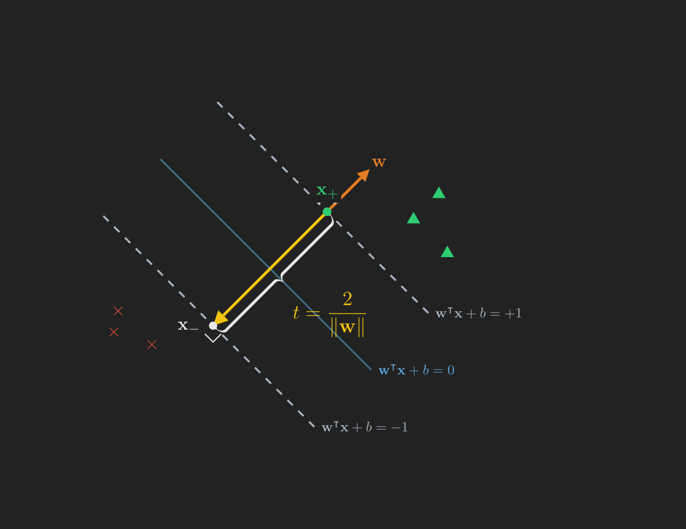
We choose \(t\) to be exactly the distance that makes \(\vb{x}_-\) land on the \(-1\) line, i.e., \(\vb{w}^{\intercal}\vb{x}_- + b = -1\). To find that \(t\), we substitute the expression for \(\vb{x}_-\) from Equation 16 into the \(-1\) line’s equation and simplify:
\[ \begin{aligned} \vb{w}^{\intercal}\vb{x}_- + b &= -1 \\ \vb{w}^{\intercal}\left(\vb{x}_+ - t\,\frac{\vb{w}}{\norm\big{\vb{w}}}\right) + b &= -1 && \text{(substitute } \vb{x}_-\text{)} \\ \underbrace{\left(\vb{w}^{\intercal}\vb{x}_+ + b\right)}_{=\,1} - t\,\frac{\vb{w}^{\intercal}\vb{w}}{\norm\big{\vb{w}}} &= -1 && \text{(distribute } \vb{w}^{\intercal}\text{)} \\ 1 - t\,\frac{\norm\big{\vb{w}}^2}{\norm\big{\vb{w}}} &= -1 && \left(\vb{w}^{\intercal}\vb{w} = \norm\big{\vb{w}}^2\right) \\ 1 - t\,\norm\big{\vb{w}} &= -1 \\ t\,\norm\big{\vb{w}} &= 2 \\ t &= \frac{2}{\norm\big{\vb{w}}}. \end{aligned} \]
Two facts did all the work: \(\vb{w}^{\intercal}\vb{x}_+ + b = 1\) (because \(\vb{x}_+\) lies on the \(+1\) line, Equation 15), and \(\vb{w}^{\intercal}\vb{w} = \norm\big{\vb{w}}^2\) (the definition of the Euclidean norm). The distance \(t\) we just travelled is the gap between the two margin lines, so the full width of the margin is
\[ \text{margin width} = t = \frac{2}{\norm\big{\vb{w}}}. \tag{17}\]
Maximizing that width means minimizing \(\norm\big{\vb{w}}\), exactly the objective in Equation 14. Figure 7 shows the finished picture: the solid boundary, the two dashed margin lines, the width \(2/\norm\big{\vb{w}}\), and, circled, the handful of points that end up touching the margin lines.
We could stop here and just call a QP solver on Equation 14. But we are going to do something that looks like a detour and turns out to be the main road. We will study the dual of this problem. The dual will (a) expose the support vectors, (b) rewrite the entire algorithm using only inner products between examples, which is precisely the doorway through which kernels enter, and (c) hand us a specialized algorithm (SMO) that beats generic QP software. To get there, we need a tool from optimization: Lagrange duality.
A Detour Through Lagrange Duality
NoteWhat this section is, and how to read it
This is a self-contained detour into constrained optimization, the machinery we need to derive the SVM’s dual form. It is general (not specific to SVMs) and a little abstract. If you want to take the results on faith, the one thing to carry forward is this: under nice (convex) conditions, a constrained minimization problem has an equivalent dual problem with the same optimal value, and the solution satisfies the KKT conditions. We follow the treatment in Ng & Ma (2023); Boyd & Vandenberghe (2004) is the definitive reference.
One notational warning before we start. Throughout this section, \(w\) denotes a generic optimization variable, an arbitrary vector we happen to be minimizing over. It is not the SVM’s weight vector \(\vb{w}\). We are proving a general theorem here and will only later apply it with \(w\) playing the role of \((\vb{w}, b)\). (This is why \(w\) is written in plain italic, not in the bold upright \(\vb{w}\) we reserve for vectors in the SVM itself.)
Warmup: Equality Constraints Only
Consider minimizing \(f(w)\) subject to equality constraints \(h_i(w) = 0\). The classical method of Lagrange multipliers forms the Lagrangian
\[ \mathcal{L}(w, \boldsymbol{\upbeta}) = f(w) + \sum_{i=1}^{l} \beta_i\, h_i(w), \tag{18}\]
where the \(\boldsymbol{\upbeta} = \begin{bmatrix} \beta_1 & \cdots & \beta_l \end{bmatrix}^{\intercal}\) are the Lagrange multipliers, and then solves \(\partial \mathcal{L}/\partial w = 0\) and \(\partial \mathcal{L}/\partial \beta_i = 0\). We now generalize this to allow inequality constraints too, which is what our SVM has.
The Primal Problem
Consider the general primal problem
\[ \begin{aligned} \min_{w} \quad & f(w) \\ \text{s.t.} \quad & g_i(w) \leq 0, \quad i = 1, \ldots, k, \\ & h_i(w) = 0, \quad i = 1, \ldots, l. \end{aligned} \tag{19}\]
We define the generalized Lagrangian
\[ \mathcal{L}(w, \boldsymbol{\upalpha}, \boldsymbol{\upbeta}) = f(w) + \sum_{i=1}^{k} \alpha_i\, g_i(w) + \sum_{i=1}^{l} \beta_i\, h_i(w), \tag{20}\]
with multipliers \(\alpha_i\) (for the inequality constraints) and \(\beta_i\) (for the equality constraints). Now here is a clever bookkeeping trick. Define
\[ \theta_{\mathcal{P}}(w) = \max_{\boldsymbol{\upalpha}, \boldsymbol{\upbeta}\,:\,\alpha_i \geq 0} \mathcal{L}(w, \boldsymbol{\upalpha}, \boldsymbol{\upbeta}), \tag{21}\]
where the subscript \(\mathcal{P}\) stands for “primal.” Consider what this maximization does for a fixed \(w\):
- If \(w\) violates some constraint (say \(g_i(w) > 0\), or \(h_i(w) \neq 0\)), the inner maximization can drive \(\mathcal{L}\) to \(+\infty\): push the offending \(\alpha_i \to +\infty\) against a positive \(g_i\), or push \(\beta_i\) toward \(\pm\infty\) against a nonzero \(h_i\). So \(\theta_{\mathcal{P}}(w) = \infty\).
- If \(w\) satisfies every constraint, the best the maximization can do is set the \(\alpha_i g_i\) terms to zero (since \(g_i \leq 0\) and \(\alpha_i \geq 0\) make each term \(\leq 0\)) and the \(\beta_i h_i\) terms are already zero. So \(\theta_{\mathcal{P}}(w) = f(w)\).
In other words,
\[ \theta_{\mathcal{P}}(w) = \begin{cases} f(w) & \text{if } w \text{ satisfies the primal constraints,}\\ \infty & \text{otherwise.} \end{cases} \tag{22}\]
Therefore minimizing \(\theta_{\mathcal{P}}\) is identical to our original constrained problem (the \(\infty\) automatically rules out infeasible \(w\)):
\[ \min_{w} \theta_{\mathcal{P}}(w) = \min_{w} \max_{\boldsymbol{\upalpha}, \boldsymbol{\upbeta}\,:\,\alpha_i \geq 0} \mathcal{L}(w, \boldsymbol{\upalpha}, \boldsymbol{\upbeta}). \tag{23}\]
Call its optimal value \(p^{*} = \min_{w} \theta_{\mathcal{P}}(w)\), the value of the primal problem.
The Dual Problem
Now swap the order of the min and the max. Define
\[ \theta_{\mathcal{D}}(\boldsymbol{\upalpha}, \boldsymbol{\upbeta}) = \min_{w} \mathcal{L}(w, \boldsymbol{\upalpha}, \boldsymbol{\upbeta}), \tag{24}\]
with \(\mathcal{D}\) for “dual.” The dual problem maximizes this over the multipliers:
\[ \max_{\boldsymbol{\upalpha}, \boldsymbol{\upbeta}\,:\,\alpha_i \geq 0} \theta_{\mathcal{D}}(\boldsymbol{\upalpha}, \boldsymbol{\upbeta}) = \max_{\boldsymbol{\upalpha}, \boldsymbol{\upbeta}\,:\,\alpha_i \geq 0} \min_{w} \mathcal{L}(w, \boldsymbol{\upalpha}, \boldsymbol{\upbeta}), \tag{25}\]
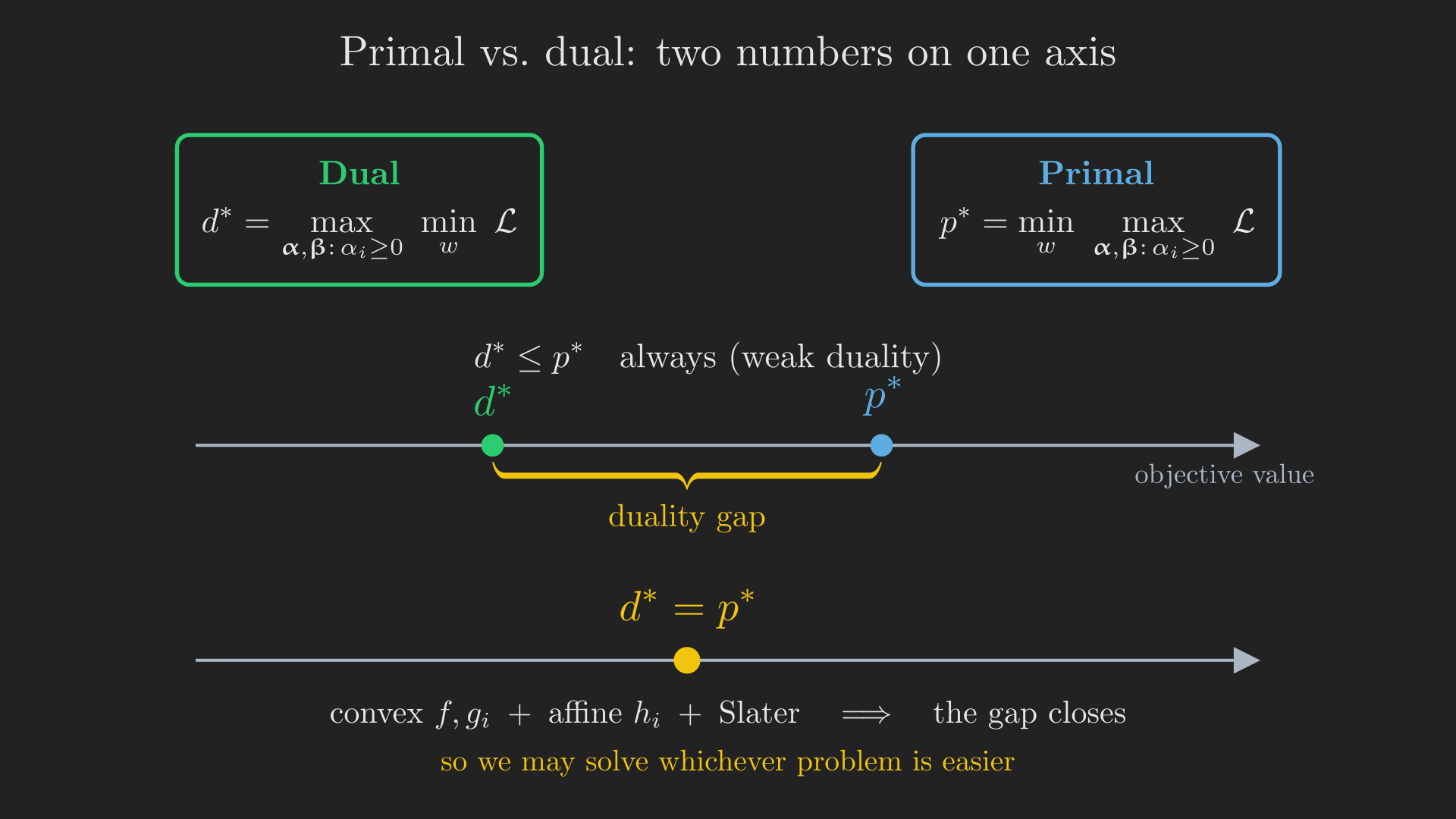
with optimal value \(d^{*}\). The primal and dual are the same expression with the “\(\max\)” and “\(\min\)” traded, as Figure 8 emphasizes.
Weak and Strong Duality
It is always true (a “max min” is never bigger than the corresponding “min max”) that
\[ \underbrace{\max_{\boldsymbol{\upalpha}, \boldsymbol{\upbeta}\,:\,\alpha_i \geq 0} \min_{w} \mathcal{L}}_{d^{*}} \;\leq\; \underbrace{\min_{w} \max_{\boldsymbol{\upalpha}, \boldsymbol{\upbeta}\,:\,\alpha_i \geq 0} \mathcal{L}}_{p^{*}}. \tag{26}\]
This is weak duality. What we really want is strong duality, \(d^{*} = p^{*}\), so that we can solve the dual instead of the primal. That holds under mild conditions: \(f\) and the \(g_i\) are convex, the \(h_i\) are affine, and the constraints are strictly feasible (there is some \(w\) with every \(g_i(w) < 0\); this is Slater’s condition). Our SVM problem Equation 14 satisfies all of these.
The KKT Conditions
Under those same conditions, there exist \(w^{*}, \boldsymbol{\upalpha}^{*}, \boldsymbol{\upbeta}^{*}\) solving the primal and dual with
\[ p^{*} = d^{*} = \mathcal{L}(w^{*}, \boldsymbol{\upalpha}^{*}, \boldsymbol{\upbeta}^{*}), \]
and they satisfy the Karush-Kuhn-Tucker (KKT) conditions:
\[ \begin{aligned} \frac{\partial}{\partial w_i}\mathcal{L}(w^{*}, \boldsymbol{\upalpha}^{*}, \boldsymbol{\upbeta}^{*}) &= 0, \quad i = 1, \ldots, d, \\ \frac{\partial}{\partial \beta_i}\mathcal{L}(w^{*}, \boldsymbol{\upalpha}^{*}, \boldsymbol{\upbeta}^{*}) &= 0, \quad i = 1, \ldots, l, \\ \alpha_i^{*}\, g_i(w^{*}) &= 0, \quad i = 1, \ldots, k, \\ g_i(w^{*}) &\leq 0, \quad i = 1, \ldots, k, \\ \alpha_i^{*} &\geq 0, \quad i = 1, \ldots, k. \end{aligned} \tag{27}\]
Conversely, any point satisfying the KKT conditions solves the primal and dual. Most of these are unsurprising (stationarity, feasibility, nonnegative multipliers). The star of the show is the third one, \(\alpha_i^{*} g_i(w^{*}) = 0\), the KKT dual-complementarity condition. It says that for each \(i\), at least one of \(\alpha_i^{*}\) and \(g_i(w^{*})\) is zero. So:
\[ \alpha_i^{*} > 0 \quad\Longrightarrow\quad g_i(w^{*}) = 0. \tag{28}\]
That is, a strictly positive multiplier forces its constraint to be active (tight, holding with equality). This one implication is about to explain why an SVM has only a few support vectors, and it will later give us a convergence test for the SMO algorithm. Keep Equation 28 in your pocket.
A Tiny Example, Before We Trust Any of This
Everything above was stated for a general \(f\), general \(g_i\), general \(h_i\). That is exactly the level of abstraction where a reader nods along without anything actually clicking. So before we turn this machinery on the SVM, let us run it on the smallest problem that exercises all of it. Solve
\[ \begin{aligned} \min_{w_1, w_2} \quad & w_1^2 + w_2^2 \\ \text{s.t.} \quad & w_1 + w_2 \geq 2. \end{aligned} \tag{29}\]
Equation 29 is easy to see geometrically, which is the point: we are looking for the point of the half-plane \(w_1 + w_2 \geq 2\) that is closest to the origin. That point is \(\left(1, 1\right)\), sitting on the boundary line, at squared distance \(2\). So we already know the answer, \(p^{*} = 2\), and can check whether duality reproduces it.
First put the constraint in the \(g(w) \leq 0\) form of Equation 19: \(g(w) = 2 - w_1 - w_2 \leq 0\). The Lagrangian, with a single multiplier \(\alpha \geq 0\), is
\[ \mathcal{L}(w, \alpha) = w_1^2 + w_2^2 + \alpha\left(2 - w_1 - w_2\right). \tag{30}\]
Now form the dual by minimizing over \(w\), exactly as Equation 24 instructs. Setting both partial derivatives to zero,
\[ \begin{align*} \pdv{\mathcal{L}}{w_1} = 2w_1 - \alpha &= 0 \implies w_1 = \frac{\alpha}{2},\\ \pdv{\mathcal{L}}{w_2} = 2w_2 - \alpha &= 0 \implies w_2 = \frac{\alpha}{2}. \end{align*} \tag{31}\]
Substituting these back into Equation 30 gives the dual objective as a function of \(\alpha\) alone:
\[ \begin{align*} \theta_{\mathcal{D}}(\alpha) &= \left(\frac{\alpha}{2}\right)^2 + \left(\frac{\alpha}{2}\right)^2 + \alpha\left(2 - \frac{\alpha}{2} - \frac{\alpha}{2}\right)\\ &= \frac{\alpha^2}{2} + 2\alpha - \alpha^2\\ &= 2\alpha - \frac{\alpha^2}{2}. \end{align*} \tag{32}\]
Maximizing Equation 32 over \(\alpha \geq 0\) is a one-variable calculus problem: \(\dv{\theta_{\mathcal{D}}}{\alpha} = 2 - \alpha = 0\), so \(\alpha^{*} = 2\), and the dual value is \(d^{*} = 2(2) - 2^2/2 = 2\).
Look at what just happened, because all three lessons of this section are visible in it at once.
- Strong duality held. We got \(d^{*} = 2 = p^{*}\). The gap in Figure 8 closed, exactly as promised, because \(f\) is convex, \(g\) is affine (hence convex), and the constraint is strictly feasible (take \(w = (5, 5)\), where \(g = -8 < 0\), satisfying Slater’s condition).
- The dual variable recovered the primal solution. Plugging \(\alpha^{*} = 2\) into Equation 31 gives \(w_1 = w_2 = 1\), the answer we read off the picture. We never optimized over \(w\) directly at the end; we optimized over \(\alpha\) and then reconstructed \(w\). That is precisely the manoeuvre the SVM is about to perform with Equation 36.
- Complementarity did what Equation 28 says. We found \(\alpha^{*} = 2 > 0\), and sure enough the constraint is active: \(w_1 + w_2 = 2\) exactly, so \(g(w^{*}) = 0\). The constraint is “pushing”, and its multiplier is positive.
That third point is worth one more moment, because it is the one the SVM leans on hardest. Suppose we had instead minimized \(w_1^2 + w_2^2\) subject to \(w_1 + w_2 \geq -2\). The unconstrained minimum \((0,0)\) already satisfies that constraint comfortably, so the constraint is doing nothing, and complementarity forces \(\alpha^{*} = 0\). A constraint that is not binding gets a zero multiplier. Hold onto that sentence: in the SVM, the constraints are the training examples, and we are about to discover that almost all of them are not binding.
The Dual Form of the SVM
Armed with duality, we return to the optimal margin classifier Equation 14 and derive its dual. This is the technical heart of the SVM, and Ng & Ma (2023) flag the punchlines as the most important takeaways of the whole chapter: the equivalence of the primal and the dual, and the formula that recovers \(\vb{w}\) from the dual variables.
First, write the constraints in the \(g_i(\vb{w}) \leq 0\) form of Equation 19:
\[ g_i(\vb{w}) = -y_i\left(\vb{w}^{\intercal}\vb{x}_i + b\right) + 1 \leq 0, \tag{33}\]
one per training example. Look at what the complementarity condition Equation 28 says here. We will have \(\alpha_i > 0\) only for examples where \(g_i(\vb{w}) = 0\), that is, where \(y_i\left(\vb{w}^{\intercal}\vb{x}_i + b\right) = 1\): examples whose functional margin is exactly 1. Those are precisely the points sitting on the margin lines in Figure 7. Every other example (strictly outside the margin) has \(\alpha_i = 0\).
ImportantSupport vectors, defined
The training examples with \(\alpha_i > 0\) are the support vectors. In the separable case we are studying here, these are exactly the few points lying on the margin boundaries: in Figure 7 there are only three (two positive, one negative). Every other example has \(\alpha_i = 0\) and contributes nothing to the model.
This is the sparsity the kernel methods post promised: the coefficient vector is mostly zeros, so at prediction time we only need to remember a handful of examples, not the whole dataset (Kharkar, 2020). It is also the “non-binding constraints get zero multipliers” lesson from our toy example, now doing real work: a training example far outside the margin is a constraint that is not pushing on anything, so its multiplier is zero and it drops out of the model entirely.
One caveat to file away: “support vector” will get slightly broader once we allow a soft margin later in this post. There, points that have crept inside the margin, or even landed on the wrong side, also carry \(\alpha_i > 0\) and count as support vectors. The clean picture of “support vectors live exactly on the margin lines” is a fact about the separable case, not the definition.
Now the derivation. As we build the dual, watch for one recurring character: the inner product \(\left\langle \vb{x}_i, \vb{x}_j \right\rangle = \vb{x}_i^{\intercal}\vb{x}_j\) between pairs of examples. The fact that the whole algorithm can be written using only these inner products is exactly what will let kernels walk in later.
The problem has only inequality constraints, so the Lagrangian uses only \(\alpha_i\) multipliers (no \(\beta_i\)):
\[ \mathcal{L}(\vb{w}, b, \boldsymbol{\upalpha}) = \frac{1}{2}\norm\big{\vb{w}}^2 - \sum_{i=1}^{n} \alpha_i\left[y_i\left(\vb{w}^{\intercal}\vb{x}_i + b\right) - 1\right]. \tag{34}\]
To find the dual \(\theta_{\mathcal{D}}(\boldsymbol{\upalpha}) = \min_{\vb{w}, b}\mathcal{L}\), we minimize over \(\vb{w}\) and \(b\) by setting the Lagrangian’s derivatives to zero. First we distribute the bracket in Equation 34 so its dependence on \(\vb{w}\) and \(b\) is explicit:
\[ \mathcal{L}(\vb{w}, b, \boldsymbol{\upalpha}) = \frac{1}{2}\vb{w}^{\intercal}\vb{w} - \sum_{i=1}^{n} \alpha_i y_i\,\vb{w}^{\intercal}\vb{x}_i - b\sum_{i=1}^{n} \alpha_i y_i + \sum_{i=1}^{n} \alpha_i. \tag{35}\]
Now differentiate Equation 35 with respect to \(\vb{w}\) and set the result to zero. Its last two terms carry no \(\vb{w}\) and drop out, while the first two use \(\grad_{\vb{w}}\!\left(\tfrac{1}{2}\vb{w}^{\intercal}\vb{w}\right) = \vb{w}\) and \(\grad_{\vb{w}}\!\left(\vb{w}^{\intercal}\vb{x}_i\right) = \vb{x}_i\):
\[ \begin{align*} \grad_{\vb{w}}\mathcal{L}(\vb{w}, b, \boldsymbol{\upalpha}) &= 0\\ \implies \grad_{\vb{w}}\!\left(\frac{1}{2}\vb{w}^{\intercal}\vb{w}\right) - \sum_{i=1}^{n} \alpha_i y_i\,\grad_{\vb{w}}\!\left(\vb{w}^{\intercal}\vb{x}_i\right) &= 0\\ \implies \vb{w} - \sum_{i=1}^{n} \alpha_i y_i\,\vb{x}_i &= 0\\ \implies \vb{w} &= \sum_{i=1}^{n} \alpha_i y_i\,\vb{x}_i. \end{align*} \tag{36}\]
This last line is the crucial formula recovering \(\vb{w}\) from the multipliers. Read it slowly: the optimal weight vector is just a weighted combination of the training examples, with weights \(\alpha_i y_i\). And since \(\alpha_i = 0\) for all non-support-vectors, only the support vectors actually appear in the sum. The boundary is literally supported by those few points; move the others and nothing changes (Kharkar, 2020).
For the intercept \(b\), only the term \(-b\sum_i \alpha_i y_i\) in Equation 35 contains \(b\). Differentiate with respect to \(b\) and set the result to zero:
\[ \begin{align*} \frac{\partial \mathcal{L}}{\partial b} &= 0\\ \implies -\sum_{i=1}^{n} \alpha_i y_i &= 0\\ \implies \sum_{i=1}^{n} \alpha_i y_i &= 0. \end{align*} \tag{37}\]
Now substitute \(\vb{w} = \sum_i \alpha_i y_i \vb{x}_i\) from Equation 36 into the expanded Lagrangian Equation 35 and simplify. Only the two \(\vb{w}\)-terms change: each turns into a double sum, and because the quadratic term is exactly half the linear one, together they leave a single \(-\tfrac{1}{2}\) double sum:
\[ \begin{align*} \mathcal{L} &= \frac{1}{2}\vb{w}^{\intercal}\vb{w} - \sum_{i=1}^{n} \alpha_i y_i\,\vb{w}^{\intercal}\vb{x}_i - b\sum_{i=1}^{n} \alpha_i y_i + \sum_{i=1}^{n} \alpha_i\\ &= \frac{1}{2}\sum_{i,j=1}^{n} y_i y_j \alpha_i \alpha_j\,\vb{x}_i^{\intercal}\vb{x}_j - \sum_{i,j=1}^{n} y_i y_j \alpha_i \alpha_j\,\vb{x}_i^{\intercal}\vb{x}_j - b\sum_{i=1}^{n} \alpha_i y_i + \sum_{i=1}^{n} \alpha_i\\ &= \sum_{i=1}^{n} \alpha_i - \frac{1}{2}\sum_{i,j=1}^{n} y_i y_j \alpha_i \alpha_j\,\vb{x}_i^{\intercal}\vb{x}_j - b\sum_{i=1}^{n} \alpha_i y_i. \end{align*} \tag{38}\]
But Equation 37 tells us the last term is zero, leaving
\[ \begin{align*} \mathcal{L}(\vb{w}, b, \boldsymbol{\upalpha}) &= \sum_{i=1}^{n} \alpha_i - \frac{1}{2}\sum_{i, j = 1}^{n} y_i y_j \alpha_i \alpha_j\, \vb{x}_i^{\intercal}\vb{x}_j\\ &= \sum_{i=1}^{n} \alpha_i - \frac{1}{2}\sum_{i, j = 1}^{n} y_i y_j \alpha_i \alpha_j \left\langle \vb{x}_i, \vb{x}_j \right\rangle. \end{align*} \tag{39}\]
Bundling this together with the constraints \(\alpha_i \geq 0\) (which we always had) and \(\sum_i \alpha_i y_i = 0\) (from Equation 37), we obtain the dual optimization problem:
\[ \begin{aligned} \max_{\boldsymbol{\upalpha}} \quad & W(\boldsymbol{\upalpha}) = \sum_{i=1}^{n} \alpha_i - \frac{1}{2}\sum_{i, j = 1}^{n} y_i y_j \alpha_i \alpha_j \left\langle \vb{x}_i, \vb{x}_j \right\rangle \\ \text{s.t.} \quad & \alpha_i \geq 0, \quad i = 1, \ldots, n, \\ & \sum_{i=1}^{n} \alpha_i y_i = 0. \end{aligned} \tag{40}\]
The SVM conditions satisfy strong duality and the KKT conditions, so we may solve Equation 40 in place of the primal Equation 14. Notice how the problem has transformed. In the primal we were solving for \(\vb{w}\) and \(b\) directly. In the dual we solve for the coefficients \(\boldsymbol{\upalpha}\), one weight per example, telling us how much each example contributes (Stanford Online, Anand Avati, 2019). (This mirrors the \(\beta_i\) coefficients from the kernel methods post, where the model was likewise a combination of the data.) Once we have the optimal \(\boldsymbol{\upalpha}\), Equation 36 recovers \(\vb{w}^{*}\), and the intercept comes from splitting the difference between the closest positive and closest negative:
\[ b^{*} = -\frac{\displaystyle\max_{i\,:\,y_i = -1} \vb{w}^{*\intercal}\vb{x}_i + \min_{i\,:\,y_i = 1} \vb{w}^{*\intercal}\vb{x}_i}{2}. \tag{41}\]
Prediction, in Inner Products
The payoff of the dual is clearest at prediction time. To classify a new test point \(\vb{x}_{\text{test}}\), we compute \(\vb{w}^{\intercal}\vb{x}_{\text{test}} + b\) and predict \(+1\) if it is positive. Using Equation 36,
\[ \begin{aligned} \vb{w}^{\intercal}\vb{x}_{\text{test}} + b &= \left(\sum_{i=1}^{n} \alpha_i y_i \vb{x}_i\right)^{\intercal}\vb{x}_{\text{test}} + b \\[0.5em] &= \sum_{i=1}^{n} \alpha_i y_i \left\langle \vb{x}_i, \vb{x}_{\text{test}} \right\rangle + b. \end{aligned} \tag{42}\]
Two things about Equation 42 are worth savoring. First, prediction depends on the input only through inner products \(\left\langle \vb{x}_i, \vb{x}_{\text{test}} \right\rangle\) between the new test point and the training points. Second, since \(\alpha_i = 0\) for all but the support vectors, almost every term vanishes; we only need inner products against the (few) support vectors. Both the training objective Equation 40 and the prediction rule Equation 42 are written entirely in inner products between data points. That is not a coincidence we stumbled into; it is the door we deliberately walked toward, because it is exactly the door kernels come through.
Checkpoint: the view from the dual
flowchart TD
    E["Maximize the margin: convex QP"] --> F["Lagrange duality + KKT"]
    F --> G["Dual form: only inner products"]
    G --> S["Sparse: only support vectors have α > 0"]
    G --> H["Next: swap inner products for kernels"]

    style G fill:#1e8449,color:#fff
    style H fill:#2471a3,color:#fff
Kernels Come Home
Everything is now in place for the trick we built in the kernel methods post. The dual objective Equation 40 and the prediction Equation 42 touch the data only through inner products \(\left\langle \vb{x}_i, \vb{x}_j \right\rangle\). So we do the one move that changes everything: replace every inner product with a kernel \(K(\vb{x}_i, \vb{x}_j) = \left\langle \boldsymbol{\upphi}(\vb{x}_i), \boldsymbol{\upphi}(\vb{x}_j) \right\rangle\). The dual becomes
\[ \begin{aligned} \max_{\boldsymbol{\upalpha}} \quad & W(\boldsymbol{\upalpha}) = \sum_{i=1}^{n} \alpha_i - \frac{1}{2}\sum_{i, j = 1}^{n} y_i y_j \alpha_i \alpha_j\, K(\vb{x}_i, \vb{x}_j) \\ \text{s.t.} \quad & \alpha_i \geq 0, \quad \sum_{i=1}^{n} \alpha_i y_i = 0, \end{aligned} \tag{43}\]
and prediction becomes
\[ \vb{w}^{\intercal}\boldsymbol{\upphi}(\vb{x}) + b = \sum_{i=1}^{n} \alpha_i y_i\, K(\vb{x}_i, \vb{x}) + b. \tag{44}\]
Without ever building a single feature vector \(\boldsymbol{\upphi}(\vb{x})\), the SVM now finds a maximum-margin boundary in the kernel’s (possibly infinite-dimensional) feature space. A linear boundary in that space corresponds to a curved boundary back in the original space. This is what lets an SVM carve out circles, wiggles, and other nonlinear shapes; a polynomial kernel handles interactions of features, and the Gaussian (RBF) kernel can fit boundaries so flexible they defy any simple description, because it secretly works in an infinite-dimensional space (Kharkar, 2020; Schölkopf & Smola, 2002). The full derivation of these kernels, and Mercer’s theorem for which functions are legal kernels, lives in the kernel methods post; here we simply enjoy the fact that they drop straight into Equation 43.
Seeing it happen
That is a large claim to make in prose, so let us watch it. Imagine a version of our admissions problem where the school is not looking for the highest scores but for the closest fit to a target profile: students near the school’s ideal GPA and MCAT combination get in, and students who are lopsided in any direction (or simply under-qualified) do not. The admitted students now form a blob in the middle, with rejected students surrounding them on all sides.
No straight line can separate that. Not one; the geometry forbids it. Figure 10 runs the very same SVM on this data three times, changing nothing except which \(K(\vb{x}_i, \vb{x}_j)\) gets substituted into Equation 43.
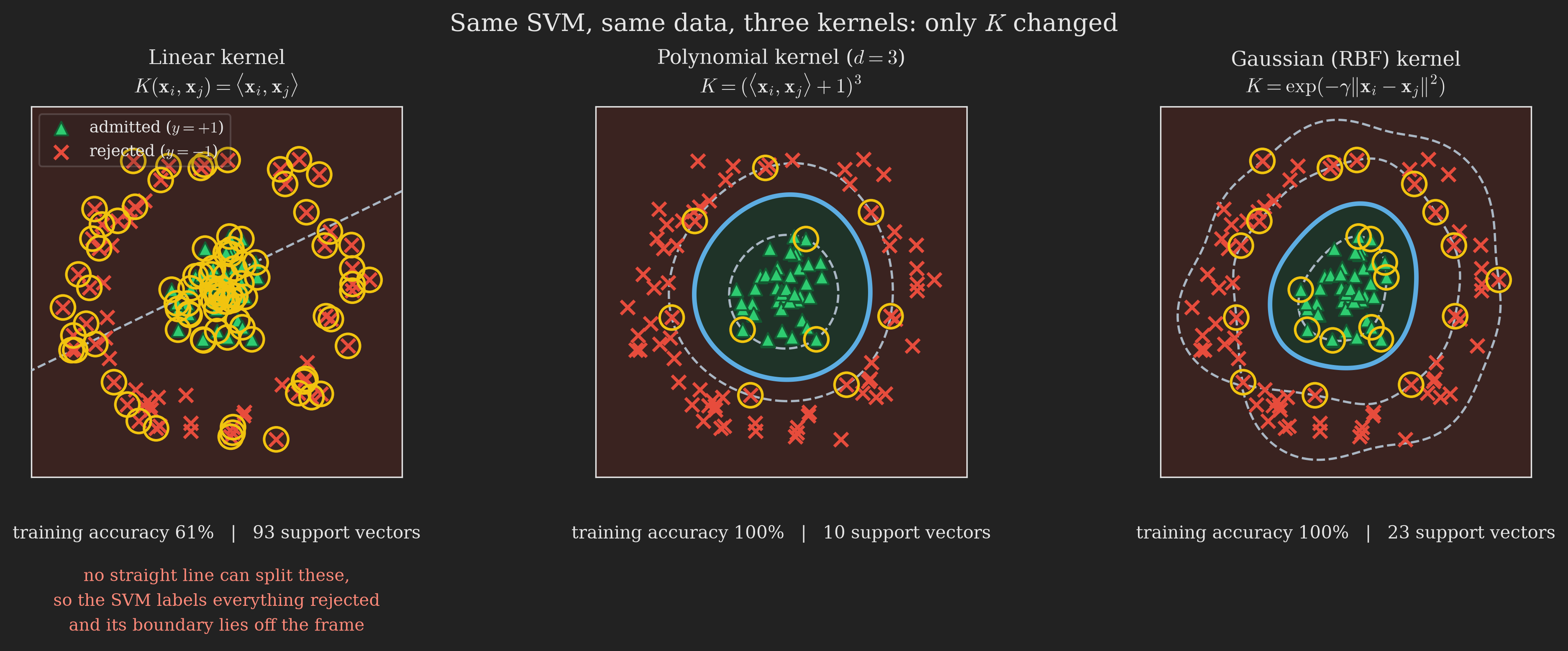
The thing to appreciate about Figure 10 is how little changed to produce it. We did not invent a new algorithm for curved boundaries. We did not write down \(\boldsymbol{\upphi}\), or compute a single feature vector, or leave two dimensions. The optimization problem is character-for-character the one we derived in Equation 40, with one symbol swapped. Every panel is still a maximum-margin linear classifier; the middle and right panels are just drawing their straight line in a space we never had to visit.
This is also the cleanest illustration of why the dual mattered. The primal Equation 14 is written in terms of \(\vb{w}\), an object that lives in feature space and would be infinite-dimensional for the RBF kernel, so it cannot even be stored. The dual Equation 40 never mentions \(\vb{w}\); it only ever asks for inner products between pairs of examples. That is the difference between an algorithm you can run and one you cannot.
There is one more reason the dual is a gift, beyond kernels, that Kharkar (2020) makes vivid. Suppose the data is high-dimensional: many features \(d\), relatively few examples \(n\) (think gene-expression data, or images with more pixels than you have images). The primal works with the raw data, an object of size \(n \times d\). The dual, by contrast, never needs the raw features; it needs only the \(n^2\) pairwise inner products (or kernel values). When \(d \gg n\), that means \(n^2 \ll nd\), so the dual is genuinely cheaper in both time and memory. High-dimensional data, which sounds like a curse, is exactly where the dual formulation shines.
So far, so clean. But we have been living in a fantasy where the data is perfectly separable. Real data is messier, and if we are not careful, our beautiful margin can be wrecked by a single bad point.
When the Data Is Not Separable
Our whole derivation assumed a separating hyperplane exists. Two things go wrong in practice. First, sometimes no straight boundary separates the classes at all (though mapping to a high-dimensional feature space via a kernel makes separability more likely, it is never guaranteed). Second, even when the data is separable, insisting on separating it perfectly can be a terrible idea, because a single outlier can drag the boundary wildly. Figure 11 shows exactly this.
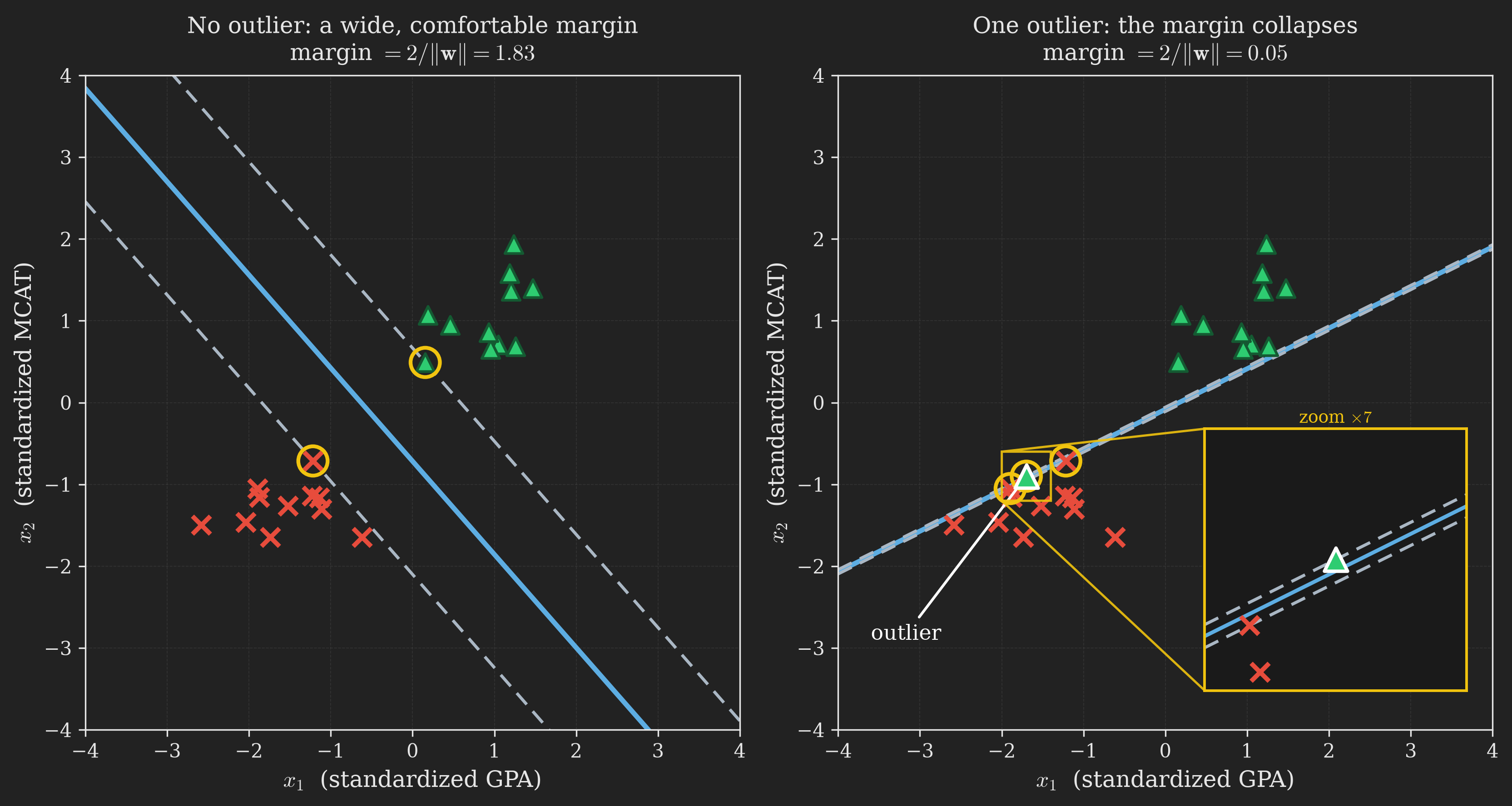
On the left, the margin is wide and the boundary sensible. On the right, we added one admitted student who, for whatever reason (there are always factors beyond GPA and MCAT), lands deep among the rejected students. The hard-margin SVM has no choice: it must classify every point correctly, so it contorts itself around the outlier, and the once-generous margin all but vanishes. Note how violent the change is: the boundary does not merely shift, it rotates by about \(75\) degrees, going from a sensible split of the two clusters to a line that runs between the outlier and its neighbours. One student out of twenty-three rewrote the entire model. We would clearly have preferred to keep the wide margin and simply tolerate one mistake (Kharkar, 2020).
The soft margin
The fix is to let examples violate the margin, but to charge them for it. We introduce a slack variable \(\xi_i \geq 0\) for each example and relax its margin constraint:
Hard margin (before):
\[ y_i\left(\vb{w}^{\intercal}\vb{x}_i + b\right) \geq 1. \tag{45}\]
Soft margin (after):
\[ y_i\left(\vb{w}^{\intercal}\vb{x}_i + b\right) \geq 1 - \xi_i. \tag{46}\]
Comparing Equation 45 with Equation 46, the slack \(\xi_i\) is simply how much of the required margin of \(1\) we are willing to forgive for example \(i\). Then we add a penalty \(C\sum_i \xi_i\) to the objective (this is called \(\ell_1\) regularization on the slacks):
\[ \begin{aligned} \min_{\vb{w}, b, \boldsymbol{\upxi}} \quad & \frac{1}{2}\norm\big{\vb{w}}^2 + C\sum_{i=1}^{n} \xi_i \\ \text{s.t.} \quad & y_i\left(\vb{w}^{\intercal}\vb{x}_i + b\right) \geq 1 - \xi_i, \quad i = 1, \ldots, n, \\ & \xi_i \geq 0, \quad i = 1, \ldots, n. \end{aligned} \tag{47}\]
An example may now have functional margin less than 1; if it has margin \(1 - \xi_i\), we pay a cost \(C\xi_i\) in the objective. Figure 12 shows the geometry of the slacks.
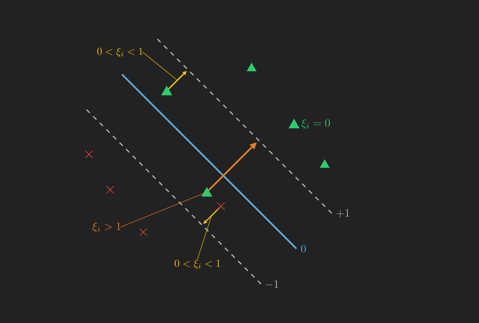
The parameter \(C > 0\) tunes the trade-off between the two goals in Equation 47: making \(\norm\big{\vb{w}}^2\) small (a wide margin) versus keeping the slacks small (few and mild violations). A large \(C\) punishes violations harshly and pushes back toward the hard margin; a small \(C\) tolerates violations in exchange for a wider, calmer margin.
That sentence is easy to write and easy to skim past, so Figure 13 shows the knob actually turning. The data here has genuinely overlapping classes (which is the honest situation whenever two test scores do not fully determine an admissions decision), so there is no hard-margin solution to fall back on and \(C\) has real work to do.
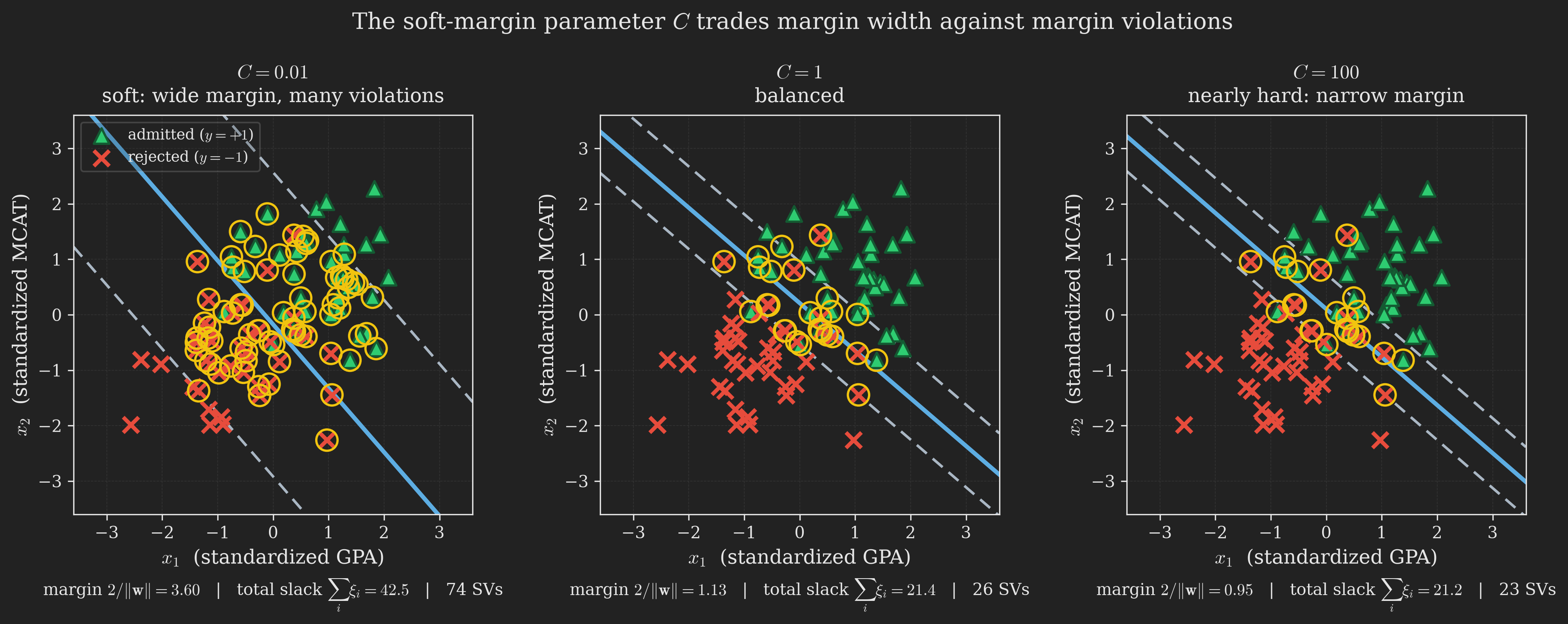
Two things in Figure 13 are worth naming explicitly. First, the support-vector count is not a fixed property of the data; it is a consequence of \(C\). Shrinking \(C\) widens the margin, which sweeps more points inside it, and every point inside the margin is a support vector. So the sparsity that makes SVMs cheap to store is itself something \(C\) trades away. Second, notice that all three panels find a similar boundary orientation. \(C\) is not choosing between wildly different explanations of the data; it is choosing how much to let the crowded middle of the dataset argue with the clean edges.
A note on why we do not penalize \(b\)
You might wonder why the objective penalizes \(\norm\big{\vb{w}}\) but leaves \(b\) alone. The reason is geometric: \(b\) controls how far the boundary sits from the origin. Penalizing \(b\) would pull the boundary toward the origin for no good reason, arbitrarily constraining where it can live. We want the algorithm free to place the boundary wherever the data demands, so we leave \(b\) unpenalized (Stanford Online, Anand Avati, 2019).
The soft-margin dual
We form the Lagrangian (now with multipliers \(\alpha_i\) for the margin constraints and \(r_i\) for the \(\xi_i \geq 0\) constraints):
\[ \mathcal{L}(\vb{w}, b, \boldsymbol{\upxi}, \boldsymbol{\upalpha}, \vb{r}) = \frac{1}{2}\vb{w}^{\intercal}\vb{w} + C\sum_{i=1}^{n} \xi_i - \sum_{i=1}^{n} \alpha_i\left[y_i\left(\vb{x}_i^{\intercal}\vb{w} + b\right) - 1 + \xi_i\right] - \sum_{i=1}^{n} r_i \xi_i. \tag{48}\]
We again minimize by setting derivatives to zero, now over \(\vb{w}\), \(b\), and \(\boldsymbol{\upxi}\). The derivatives with respect to \(\vb{w}\) and \(b\) reproduce exactly what they gave in the separable case, Equation 36 and Equation 37, so the only genuinely new ingredient is the derivative with respect to each slack \(\xi_i\). In Equation 48 the slack \(\xi_i\) appears only in \(C\xi_i\), \(-\alpha_i \xi_i\), and \(-r_i \xi_i\), so we differentiate with respect to it and set the result to zero:
\[ \begin{align*} \frac{\partial \mathcal{L}}{\partial \xi_i} &= 0\\ \implies C - \alpha_i - r_i &= 0\\ \implies \alpha_i &= C - r_i. \end{align*} \tag{49}\]
Because the multiplier \(r_i \geq 0\), Equation 49 forces \(\alpha_i \leq C\), and that is the only new restriction. Substituting everything back in as before gives a dual almost identical to the separable case:
\[ \begin{aligned} \max_{\boldsymbol{\upalpha}} \quad & W(\boldsymbol{\upalpha}) = \sum_{i=1}^{n} \alpha_i - \frac{1}{2}\sum_{i, j = 1}^{n} y_i y_j \alpha_i \alpha_j \left\langle \vb{x}_i, \vb{x}_j \right\rangle \\ \text{s.t.} \quad & 0 \leq \alpha_i \leq C, \quad i = 1, \ldots, n, \\ & \sum_{i=1}^{n} \alpha_i y_i = 0. \end{aligned} \tag{50}\]
Compare it to the hard-margin dual Equation 40 and marvel at how little changed:
Hard margin:
\[ \alpha_i \geq 0. \]
Soft margin:
\[ 0 \leq \alpha_i \leq C. \]
That is the only difference: the multipliers now have an upper bound \(C\). The objective is unchanged, \(\vb{w}\) is still recovered from Equation 36, and prediction still uses Equation 42 (kernels still plug straight in).
The intercept formula Equation 41 does need modifying, and it is worth seeing how rather than being sent away for it, because the fix falls straight out of the conditions we are about to write down. Call a support vector free if \(0 < \alpha_i < C\), that is, it is neither ignored nor pinned at the cap. For any such example the KKT conditions (Equation 52 below) give \(y_i\left(\vb{w}^{\intercal}\vb{x}_i + b\right) = 1\) exactly. Multiplying through by \(y_i\) and using \(y_i^2 = 1\), we can solve for the intercept directly:
\[ b = y_i - \vb{w}^{\intercal}\vb{x}_i \quad \text{for any free support vector } i. \tag{51}\]
In exact arithmetic every free support vector returns the same \(b\). In floating point they differ slightly, so the standard practice is to average Equation 51 over all of them. Platt’s paper covers how to maintain \(b\) incrementally while the algorithm runs, which is a separate and more delicate problem (Platt, 1998).
The KKT conditions, softened
The dual-complementarity conditions now read (these become our SMO convergence test):
\[ \begin{aligned} \alpha_i = 0 &\;\Longrightarrow\; y_i\left(\vb{w}^{\intercal}\vb{x}_i + b\right) \geq 1, \\ \alpha_i = C &\;\Longrightarrow\; y_i\left(\vb{w}^{\intercal}\vb{x}_i + b\right) \leq 1, \\ 0 < \alpha_i < C &\;\Longrightarrow\; y_i\left(\vb{w}^{\intercal}\vb{x}_i + b\right) = 1. \end{aligned} \tag{52}\]
Table 1 reads these off in plain language: they classify each example by where it sits relative to the margin.
| Multiplier | Meaning | Where the example sits |
|---|---|---|
| \(\alpha_i = 0\) | not a support vector | strictly outside the margin (correct, confident) |
| \(0 < \alpha_i < C\) | support vector on the margin | exactly on its margin line |
| \(\alpha_i = C\) | support vector inside/over the margin | inside the margin or misclassified |
The Hinge Loss View
There is a second, equivalent way to write the soft-margin SVM that connects it to the loss-function view of machine learning, and it is the form you will most often meet in practice (Kharkar, 2020; Stanford Online, Anand Avati, 2019). Look again at the slack constraints in Equation 47. For a fixed \((\vb{w}, b)\), the cheapest legal choice of each slack is
\[ \xi_i = \max\left(0,\; 1 - y_i\left(\vb{w}^{\intercal}\vb{x}_i + b\right)\right), \tag{53}\]
because \(\xi_i\) must be at least \(1 - y_i(\vb{w}^{\intercal}\vb{x}_i + b)\) (from the margin constraint) and at least \(0\), and making it any larger only wastes objective. Substituting Equation 53 into Equation 47 turns the constrained problem into an unconstrained one:
\[ \min_{\vb{w}, b} \quad \frac{1}{2}\norm\big{\vb{w}}^2 + C\sum_{i=1}^{n} \max\left(0,\; 1 - y_i\left(\vb{w}^{\intercal}\vb{x}_i + b\right)\right). \tag{54}\]
The quantity \(\max\left(0, 1 - y_i(\vb{w}^{\intercal}\vb{x}_i + b)\right)\) is the famous hinge loss (also called the SVM loss). Writing \(m = y\left(\vb{w}^{\intercal}\vb{x} + b\right)\) for the functional margin (“the score times the true label”), the hinge loss is \(\max(0, 1 - m)\), plotted in Figure 14.
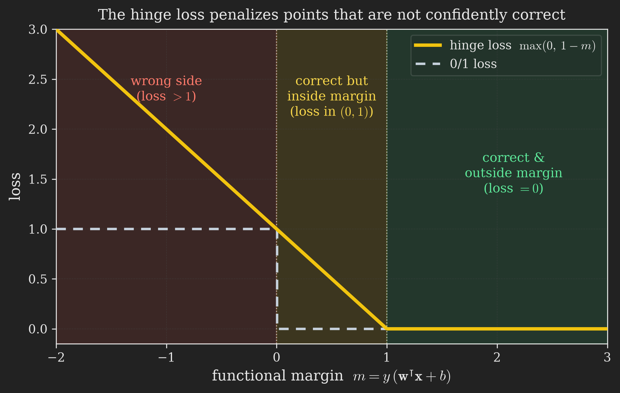
The shape tells the whole story of what an SVM wants (Kharkar, 2020). Walk through a few examples with \(y_i\) the true label and the “score” \(\vb{w}^{\intercal}\vb{x}_i + b\):
- A confidently-correct point (\(m > 1\), safely outside the margin) pays zero loss. The SVM is happy and asks nothing more of it. This is the flat part of the hinge.
- A correct-but-timid point (\(0 < m < 1\), inside the margin) pays a small loss between 0 and 1. It is classified correctly, but the SVM is not comfortable that it sits so close to the boundary, so it nudges.
- A misclassified point (\(m < 0\), wrong side) pays a large loss greater than 1, growing the deeper into the wrong side it goes. Bigger mistakes cost more.
Notice what Equation 54 is really saying. The first term \(\tfrac{1}{2}\norm\big{\vb{w}}^2\) is the same margin-maximizing pressure as before (small \(\norm\big{\vb{w}}\) means wide margin). The second term is the total hinge loss, the price of misclassifications and margin violations. The constant \(C\) balances them, just as before. And here is a subtle but important point about why we prefer Equation 47 or Equation 54 over trying to optimize something more naive: the hinge form’s \(\max\) is not differentiable at the kink, which is awkward, but both forms are convex, so we can hand them to reliable convex solvers (Boyd & Vandenberghe, 2004; Stanford Online, Anand Avati, 2019). The regularizer \(\tfrac{1}{2}\norm\big{\vb{w}}^2\) also does real work: it stops the model from cheating by scaling \(\vb{w}\) up to inflate the functional margin, exactly the loophole we identified back in Equation 3.
Checkpoint: three faces of the same model
We have picked up a lot since the last checkpoint, and it is worth pausing to see that the pieces are not three separate models but three views of one.
flowchart TD
    G["Dual form: only inner products"] --> H["Kernels: nonlinear boundaries"]
    H --> I["Soft margin: cap the multipliers at C"]
    I --> P["Primal QP"]
    I --> Q["Hinge loss (unconstrained)"]
    I --> R["Dual QP (kernels plug in here)"]
    R --> J["Next: solve it with SMO"]

    style I fill:#1e8449,color:#fff
    style J fill:#2471a3,color:#fff
TipThe same classifier, written three ways
- Primal QP Equation 47: minimize \(\tfrac{1}{2}\norm\big{\vb{w}}^2 + C\sum_i \xi_i\) subject to margin constraints. Best for understanding what we are asking for, since the margin and the violations are both explicit.
- Hinge loss Equation 54: minimize \(\tfrac{1}{2}\norm\big{\vb{w}}^2 + C\sum_i \max\left(0, 1 - y_i\left(\vb{w}^{\intercal}\vb{x}_i + b\right)\right)\), with no constraints at all. Best for connecting the SVM to the rest of machine learning, where “regularizer plus loss” is the universal template.
- Dual QP Equation 50: maximize \(W(\boldsymbol{\upalpha})\) over \(0 \leq \alpha_i \leq C\) with \(\sum_i \alpha_i y_i = 0\). Best for actually computing, since it is the only one of the three that admits kernels and reveals the support vectors.
They have the same solution. Which one you write down is a question of what you want to see.
All that remains is to actually solve the dual efficiently. That is the job of the SMO algorithm.
Solving the Dual: The SMO Algorithm
The dual Equation 50 is a QP, and generic QP software can solve it. But John Platt’s SMO (Sequential Minimal Optimization) algorithm does much better by exploiting the problem’s special structure (Platt, 1998). To motivate SMO, we first meet its simpler cousin, coordinate ascent.
Coordinate ascent
Suppose we want to maximize some function \(W(\alpha_1, \ldots, \alpha_n)\) (forget the SVM for a moment; think of \(W\) as any function). We have already met gradient descent and Newton’s method. Coordinate ascent is a third idea, almost embarrassingly simple: optimize one variable at a time, holding all others fixed.
Algorithm 1
\begin{algorithm}
\caption{Coordinate Ascent}
\begin{algorithmic}
\STATE Initialize $\boldsymbol{\upalpha}$
\WHILE{not converged}
    \FOR{$i = 1$ \TO $n$}
        \STATE $\alpha_i \gets \operatorname*{arg\,max}_{\hat{\alpha}_i}\; W(\alpha_1, \ldots, \alpha_{i-1}, \hat{\alpha}_i, \alpha_{i+1}, \ldots, \alpha_n)$
    \ENDFOR
\ENDWHILE
\end{algorithmic}
\end{algorithm}
In the inner loop, we freeze every variable except \(\alpha_i\) and re-optimize \(W\) over just \(\alpha_i\). When that one-variable maximization is easy to do in closed form, coordinate ascent can be very efficient. Figure 16 shows it in action on a quadratic.
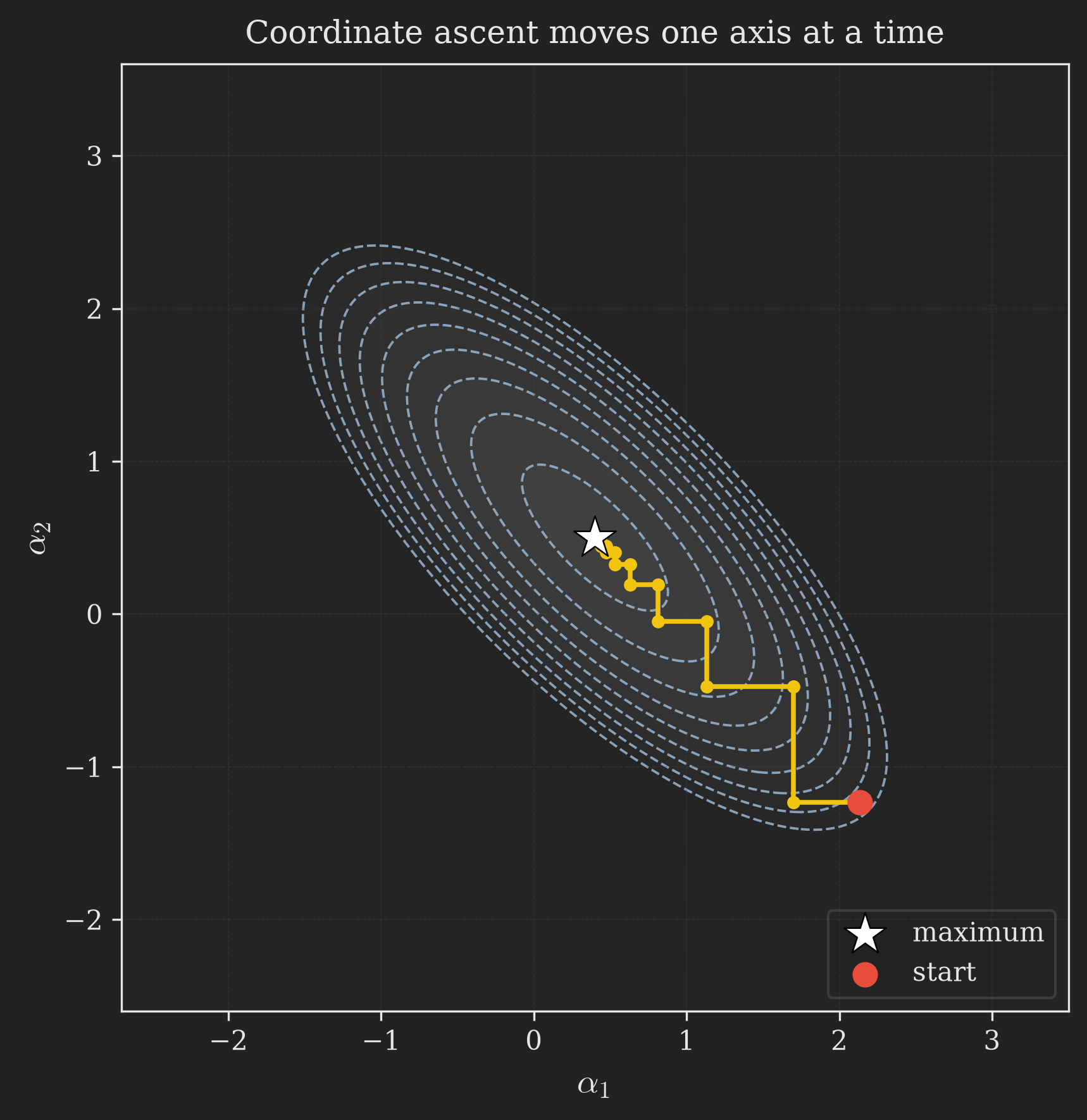
Each step moves parallel to an axis, since only one coordinate changes at a time. It is this “optimize a tiny piece at a time” spirit that SMO inherits.
SMO
Can we just apply coordinate ascent directly to the SVM dual Equation 50? Not quite, and the reason is instructive. The dual has the equality constraint \(\sum_{i=1}^{n} \alpha_i y_i = 0\). Suppose we try to update \(\alpha_1\) alone, holding \(\alpha_2, \ldots, \alpha_n\) fixed. The constraint says
\[ \alpha_1 y_1 = -\sum_{i=2}^{n} \alpha_i y_i, \tag{55}\]
and multiplying both sides by \(y_1\) (using \(y_1^2 = 1\) since \(y_1 \in \{-1, 1\}\)) shows that \(\alpha_1\) is completely determined by the others. We cannot budge \(\alpha_1\) without violating the constraint. So single-variable updates are impossible here.
The fix is the “minimal” in Sequential Minimal Optimization: update the smallest number of variables that preserves the constraint, which is two at a time.
Algorithm 2
\begin{algorithm}
\caption{SMO (Sequential Minimal Optimization)}
\begin{algorithmic}
\WHILE{not converged (KKT conditions not satisfied to within $tol$)}
    \STATE Select a pair $\alpha_i, \alpha_j$ to update (heuristic: pick the pair promising the most progress)
    \STATE Reoptimize $W(\boldsymbol{\upalpha})$ over $\alpha_i, \alpha_j$, holding all other $\alpha_k$ ($k \neq i, j$) fixed
\ENDWHILE
\end{algorithmic}
\end{algorithm}
To test convergence we check whether the KKT conditions Equation 52 hold to within a tolerance \(tol\) (typically around \(0.01\) to \(0.001\)) (Platt, 1998). The reason SMO is fast is that the two-variable update in alg. 2 can be solved analytically, in closed form. Here is the idea.
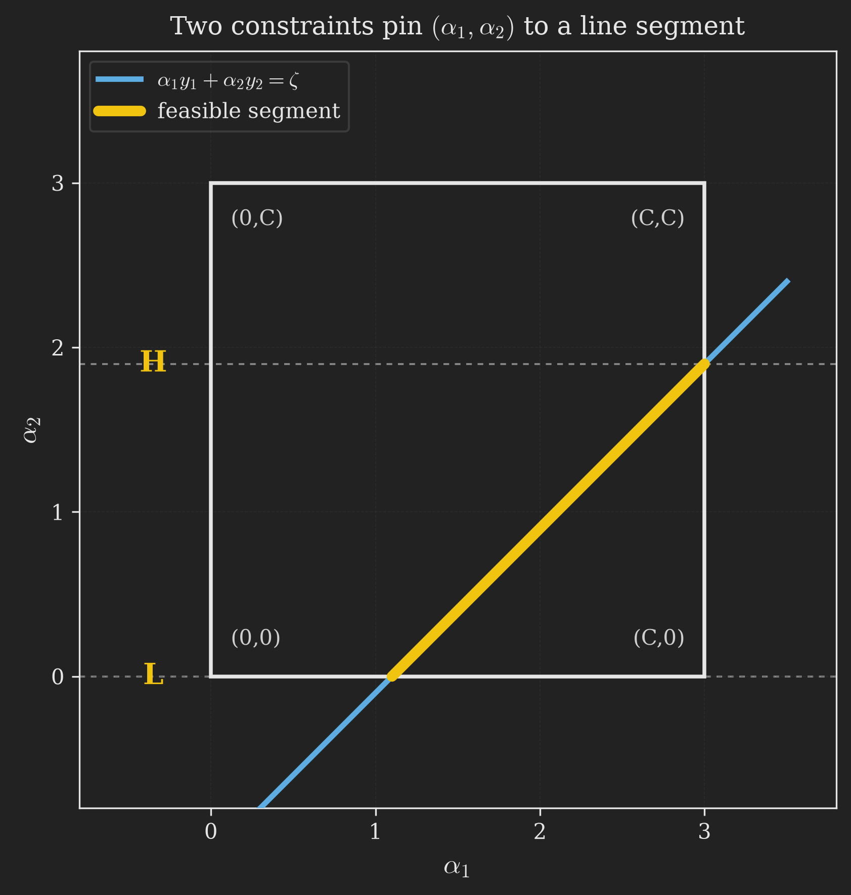
Say we hold \(\alpha_3, \ldots, \alpha_n\) fixed and reoptimize over \(\alpha_1\) and \(\alpha_2\). The equality constraint pins their combination to a constant:
\[ \alpha_1 y_1 + \alpha_2 y_2 = -\sum_{i=3}^{n} \alpha_i y_i = \zeta, \tag{56}\]
where \(\zeta\) is fixed. Together with the box constraints \(0 \leq \alpha_1, \alpha_2 \leq C\), this confines \((\alpha_1, \alpha_2)\) to a line segment, the intersection of the diagonal line Equation 56 with the box \([0, C] \times [0, C]\). Figure 17 shows exactly this feasible set.
From Equation 56 we can write \(\alpha_1\) as a function of \(\alpha_2\):
\[ \alpha_1 = \left(\zeta - \alpha_2 y_2\right) y_1 \tag{57}\]
(again using \(y_1^2 = 1\)). Substituting into \(W\) leaves a function of the single variable \(\alpha_2\), and because \(W\) is quadratic, this is just a one-variable quadratic \(p\,\alpha_2^2 + q\,\alpha_2 + r\) for some constants \(p\), \(q\), \(r\) built from the data. (We deliberately do not call them \(a\), \(b\), \(c\) here: \(b\) is already the intercept, and reusing it for a quadratic coefficient in the same post would be asking for trouble.) Ignoring the box for a moment, we maximize it by setting the derivative to zero, giving an unconstrained optimum we call \(\alpha_2^{\text{new, unclipped}}\). Then we honor the box by simply clipping that value into the allowed interval \([L, H]\):
\[ \alpha_2^{\text{new}} = \begin{cases} H & \text{if } \alpha_2^{\text{new, unclipped}} > H, \\ \alpha_2^{\text{new, unclipped}} & \text{if } L \leq \alpha_2^{\text{new, unclipped}} \leq H, \\ L & \text{if } \alpha_2^{\text{new, unclipped}} < L. \end{cases} \tag{58}\]
What exactly are \(L\) and \(H\)? They are the ends of the highlighted segment in Figure 17: the smallest and largest values \(\alpha_2\) can take while keeping both multipliers inside \([0, C]\). They depend on whether the two labels agree, because that determines whether the constraint line has slope \(+1\) or \(-1\):
\[ \begin{aligned} y_1 \neq y_2 \;(\text{slope } +1): \quad & L = \max\left(0,\; \alpha_2 - \alpha_1\right), \quad && H = \min\left(C,\; C + \alpha_2 - \alpha_1\right),\\ y_1 = y_2 \;(\text{slope } -1): \quad & L = \max\left(0,\; \alpha_1 + \alpha_2 - C\right), \quad && H = \min\left(C,\; \alpha_1 + \alpha_2\right), \end{aligned} \tag{59}\]
where \(\alpha_1\) and \(\alpha_2\) on the right-hand sides are the current values, before the update. Both cases in Equation 59 can be read straight off the picture: the line \(\alpha_1 y_1 + \alpha_2 y_2 = \zeta\) enters and leaves the box somewhere, and \(L\) and \(H\) are just the \(\alpha_2\)-coordinates of those two crossings. In Figure 17, \(H\) comes from the line exiting through the right edge (\(\alpha_1 = C\)) rather than the top, which is why \(H < C\) there.
Finally, Equation 56 recovers \(\alpha_1^{\text{new}}\) from \(\alpha_2^{\text{new}}\). Because each step is a tiny closed-form clip-and-solve, SMO rips through the dual far faster than a generic QP solver would. Two remaining details, the heuristic for choosing which pair \((\alpha_i, \alpha_j)\) to update and how to update the intercept \(b\) as the algorithm runs, are handled carefully in Platt’s paper (Platt, 1998).
The Whole Thing, in Twenty Lines of Code
We have derived a lot on paper. Before closing, let us run it, on the very same admissions data we drew back in Figure 1, and check that the objects we spent this post deriving are really there.
First, rebuild the data and fit a hard-margin SVM. (Setting \(C\) enormous makes violations effectively forbidden, which recovers the hard margin of Equation 14; there is no separate “hard margin” switch, because the hard margin is just the soft margin with an infinite price on slack.)
Code
import numpy as np
from sklearn.svm import SVC

def make_admissions_data(seed=7, n=11, gap=0.6, scale=0.55):
    """Two separable clouds: admitted students upper-right, rejected lower-left."""
    rng = np.random.default_rng(seed)
    pos, neg = [], []
    while len(pos) < n:
        p = rng.normal([1.2, 1.2], scale, size=2)
        if p[0] + p[1] > gap:
            pos.append(p)
    while len(neg) < n:
        p = rng.normal([-1.2, -1.2], scale, size=2)
        if p[0] + p[1] < -gap:
            neg.append(p)
    return np.array(pos), np.array(neg)

pos, neg = make_admissions_data()
X = np.vstack([pos, neg])
y = np.hstack([np.ones(len(pos)), -np.ones(len(neg))])

clf = SVC(kernel="linear", C=1e6).fit(X, y)
w, b = clf.coef_[0], clf.intercept_[0]

print(f"n training examples : {len(X)}")
print(f"w                   : {np.round(w, 4)}")
print(f"b                   : {b:.4f}")
print(f"margin 2/||w||      : {2 / np.linalg.norm(w):.4f}")
print(f"support vectors     : {len(clf.support_vectors_)} of {len(X)}")
n training examples : 22
w : [0.8233 0.7226]
b : 0.5183
margin 2/||w|| : 1.8258
support vectors : 2 of 22That margin of about \(1.83\) is the same number printed on the left panel of Figure 11, which is reassuring: the figure and the formula agree.
But look at the last line. Out of twenty-two students, two are support vectors. The other twenty could be deleted from the dataset and the boundary would not move a millimetre. That is Equation 28, the KKT dual-complementarity condition, showing up as a concrete number rather than as a claim.
Now let us verify the single most important formula in this post, Equation 36, which said \(\vb{w} = \sum_i \alpha_i y_i \vb{x}_i\). In scikit-learn the products \(\alpha_i y_i\) for the support vectors are stored in dual_coef_, so we can rebuild \(\vb{w}\) by hand and compare:
Code
alpha_y = clf.dual_coef_[0]             # this is alpha_i * y_i, support vectors only
alpha = np.abs(alpha_y)                 # ... so |alpha_i * y_i| = alpha_i, since y_i = +/-1

# eq-w_from_alpha, computed by hand from the dual variables:
w_rebuilt = (alpha_y[:, None] * clf.support_vectors_).sum(axis=0)

print(f"alpha_i (support vectors) : {np.round(alpha, 4)}")
print(f"w from sklearn            : {np.round(w, 6)}")
print(f"w rebuilt by hand         : {np.round(w_rebuilt, 6)}")
print(f"identical?                : {np.allclose(w, w_rebuilt)}")

# The dual's equality constraint, eq-b_constraint:
alpha_full = np.zeros(len(X))
alpha_full[clf.support_] = alpha
print(f"sum_i alpha_i y_i         : {(alpha_full * y).sum():.2e}   (should be 0)")

# eq-b_soft: any free support vector recovers the intercept.
i = clf.support_[0]
print(f"b from y_i - w.x_i        : {y[i] - w @ X[i]:.4f}   (sklearn: {b:.4f})")
alpha_i (support vectors) : [0.6 0.6]
w from sklearn : [0.823311 0.722588]
w rebuilt by hand : [0.823311 0.722588]
identical? : True
sum_i alpha_i y_i : 0.00e+00 (should be 0)
b from y_i - w.x_i : 0.5183 (sklearn: 0.5183)Every equation we derived is in that output. The weight vector really is a weighted sum of a handful of training examples. The multipliers really do satisfy \(\sum_i \alpha_i y_i = 0\). The intercept really can be read off any free support vector. None of this is scikit-learn being clever; it is Equation 36, Equation 37, and Equation 51.
Finally, the punchline of the kernel section. To get from a straight boundary to the curved ones in Figure 10, we change one keyword argument:
Code
# Admitted students near a target profile; rejected ones surrounding them.
rng = np.random.default_rng(3)
r_in, th_in = rng.uniform(0, 1.05, 45), rng.uniform(0, 2 * np.pi, 45)
r_out, th_out = rng.uniform(1.85, 2.75, 70), rng.uniform(0, 2 * np.pi, 70)
Xk = np.vstack([
    np.column_stack([r_in * np.cos(th_in), r_in * np.sin(th_in)]),
    np.column_stack([r_out * np.cos(th_out), r_out * np.sin(th_out)]),
])
yk = np.hstack([np.ones(45), -np.ones(70)])

for kernel, kwargs in [("linear", {}),
                       ("poly", {"degree": 3, "coef0": 1.0}),
                       ("rbf", {"gamma": 0.8})]:
    m = SVC(kernel=kernel, C=1.0, **kwargs).fit(Xk, yk)
    print(f"{kernel:>6} kernel : accuracy {m.score(Xk, yk):.0%}, "
          f"{len(m.support_vectors_)} support vectors")
linear kernel : accuracy 61%, 93 support vectors
poly kernel : accuracy 100%, 10 support vectors
rbf kernel : accuracy 100%, 23 support vectorsThe linear kernel cannot do better than guessing the majority class, because no straight line separates a blob from the ring around it. Swap in a polynomial or Gaussian kernel and the same solver, the same dual problem, and the same margin-maximizing principle separate the data perfectly. That is the whole payoff of having written everything in inner products.
Conclusion: What We Gained, and Where We Go Next
Let us close the loop we opened with three lines through some medical-school data.
Back at Figure 1 we eyeballed three candidate boundaries and felt that \(L_2\) was best. We can now say precisely what that feeling was measuring, and we have checked it twice over: the corridor around \(L_2\) was \(0.91\) wide against \(0.10\) for its rivals, and when we finally handed the same data to a solver, it returned a margin of \(1.83\), which is \(2 \times 0.91\), exactly the \(2/\norm\big{\vb{w}}\) of Equation 17. The instinct and the arithmetic are the same thing. Two of the twenty-two students turned out to determine that boundary entirely.
We began with a purely visual instinct, prefer the boundary with the most breathing room, and turned it into mathematics. “Breathing room” became the geometric margin; the raw functional margin looked tempting but could be gamed by rescaling, so we normalized it away. Maximizing the margin became a clean convex quadratic program, the optimal margin classifier Equation 14. Rather than solve it directly, we detoured through Lagrange duality and the KKT conditions, and that detour paid off three times over:
- The dual form Equation 40 exposed the support vectors, the few points on the margin that alone determine the boundary, making the model sparse and cheap to store.
- It rewrote everything in inner products, so kernels Equation 43 drop straight in and give us nonlinear boundaries in vast feature spaces for free.
- It handed us a specialized solver, SMO alg. 2, that beats generic QP software.
Then we made the method survive contact with reality. A single outlier can wreck a hard margin, so we introduced slack variables and the soft margin Equation 47, whose only effect on the dual was to cap the multipliers at \(C\). We saw the same idea from the loss-function angle as the hinge loss Equation 54, which charges points for being unconfident or wrong.
The result is the support vector machine: a maximum-margin classifier that pairs naturally with kernels, keeps only the examples that matter, and is trained by an efficient, purpose-built algorithm. For decades it was, and for many tabular and medium-sized problems still is, one of the most reliable off-the-shelf classifiers available (Cortes & Vapnik, 1995).
Two honest limitations to carry away. First, prediction cost scales with the number of support vectors, the issue we flagged in the kernel methods post, so on truly massive datasets methods like deep neural networks (whose cost does not grow with stored examples) tend to take over. And as Figure 13 showed, that cost is not fixed: a small \(C\) can turn most of your training set into support vectors.
Second, everything in this post was binary. The margin, the labels \(y \in \{-1, +1\}\), the single boundary: all of it assumes exactly two classes. For \(k\) classes the standard workarounds are one-vs-rest (train \(k\) classifiers, each separating one class from all the others, and take the most confident) and one-vs-one (train \(\binom{k}{2}\) classifiers on every pair and vote). Neither is as elegant as the theory above, and both are what scikit-learn is quietly doing when you hand SVC three or more classes.
If you want to go deeper, three threads beckon: the kernel methods post for the full theory of kernels and Mercer’s theorem; Platt’s paper for the nuts and bolts of SMO (Platt, 1998); and the standard references (Bishop, 2006; Hastie et al., 2009; Schölkopf & Smola, 2002) for the broader statistical-learning picture. But the core idea you can carry anywhere is the one we started with: when you must draw a line between two classes, draw the one that leaves the most room, and let the few points nearest the frontier do the supporting.
References
Bishop, C. M. (2006). Pattern Recognition and Machine Learning. Springer.
Boyd, S., & Vandenberghe, L. (2004). Convex Optimization. Cambridge University Press.
Cortes, C., & Vapnik, V. (1995). Support-Vector Networks. Machine Learning, 20(3), 273–297. https://doi.org/10.1007/BF00994018
Hastie, T., Tibshirani, R., Friedman, J., et al. (2009). The Elements of Statistical Learning: Data Mining, Inference, and Prediction. Springer series in statistics New-York.
Kharkar, R. (2020). Support Vector Machines and Kernels (Data Science Concepts video series). YouTube video series. https://www.youtube.com/@ritvikmath
Ng, A., & Ma, T. (2023). CS229 Lecture Notes. Stanford University; https://cs229.stanford.edu/main_notes.pdf.
Platt, J. C. (1998). Sequential Minimal Optimization: A Fast Algorithm for Training Support Vector Machines (Nos. MSR-TR-98-14). Microsoft Research.
Schölkopf, B., & Smola, A. J. (2002). Learning with Kernels: Support Vector Machines, Regularization, Optimization, and Beyond. MIT Press.
Stanford Online, Anand Avati. (2019). Stanford CS229: Machine Learning Course | Summer 2019. Stanford University; https://youtube.com/playlist?list=PLoROMvodv4rNH7qL6-efu_q2_bPuy0adh.
Footnotes
You may know linear programming, which minimizes a linear objective subject to linear constraints. Quadratic programming allows a convex quadratic objective (like our \(\tfrac{1}{2}\norm\big{\vb{w}}^2\)) with linear constraints, and good QP software is widely available.↩︎